
Exploration 08
텍스트 요약(Text Summarization)이란?

텍스트 요약(Text Summarization)이란
위 그림과 같이 긴 길이의 문서(Document)원문을 핵심 주제만으로 구성된 짧은 요약(Summary)문장들로 변환하는 것을 말한다.
텍스트 요약시 주의할 점
- 요약 전후에 정보 손실 발생이 최소화되야한다.
- 즉, 텍스트의 길이가 크게 줄어들었지만, 요약문은 문서 원문이 담고 있는 정보를 최대한 보존하고 있어야한다.
텍스트 요약 방법
- 추출적 요약(Extractive Summarization)
- 추상적 요약(Abstractive Summarization)
추출적 요약(Extractive Summarization)
추출적 요약이란?
단어 그대로 원문에서 문장들을 추출해서 요약하는 방식
ex. 10개의 문장이 있다면 그 중 3개의 문장을 추출하는 방식
- 문제점: 꺼내온 문장들 간의 호응이 자연스럽지 않을 수 있다.
- 알고리즘: 텍스트 랭크(TextRank)
- 자연어 처리 분야: 문장 분류(Text Classification)
추상적 요약(Abstractive Summarization)
추상적 요약이란?
원문으로부터 내용이 요약된 새로운 문장을 생성해내는 방식
- 자연어 처리 분야: 자연어 생성(Natural Language Generation, NLG)
인공 신경망으로 텍스트 요약 훈련시키기
seq2seq모델을 이용하여 Abstractive summarization방식의 텍스트 요약기를 만들어 보자.
seq2seq모델이란?
seq2seq모델은 두 개의 RNN 아키텍처를 사용하여 입력 시퀀스로부터 출력 시퀀스를 생성해 내는 자연어 생성 모델이다.
seq2seq 개요

컨텍스트 벡터(context vector)란?
원문을 첫 번째 RNN인 인코더로 입력하면, 인코더는 이를 하나의 문맥정보를 가지고 있는 고정된 벡터로 변환하는데 이를 컨텍스트 벡터라고 한다.
- 인코더: 원문을 하나의 컨텍스트 벡터로 변환
- 디코더: 컨텍스트 벡터를 전달받아 한 단어씩 생성해내서 요약 문장을 완성
LSTM과 컨텍스트 벡터

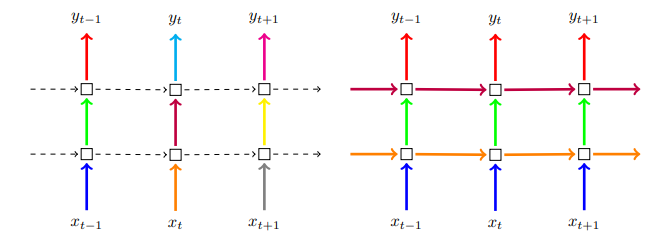
LSTM vs 바닐라 RNN
- LSTM은 다음 time step의 셀에 hidden state뿐만 아니라, cell state도 함께 전달한다. 다시 말해 인코더가 디코더에 전달하는 컨텍스트 벡터 또한 hidden state와 cell state 두 개의 값 모두 존재해야 한다.
시작 토큰과 종료 토큰
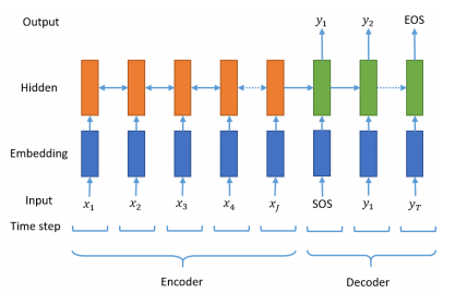
- 시작 토큰 SOS가 입력되면, 각 시점마다 단어를 생성하고 이 과정을 종료 토큰 EOS를 예측하는 순간까지 멈추지 않는다.
어텐션 메커니즘을 통한 새로운 컨텍스트 벡터 사용하기

기존의 seq2seq는 인코더의 마지막 time step의 hidden state를 컨텍스트 벡터로 사용
→ 문제점: 컨텍스트 정보에는 이미 입력 시퀀스의 많은 정보가 손실이 된 상태가 된다.
어텐션 메커니즘이란?
인코더의 모든 step의 hidden state의 정보가 컨텍스트 벡터에 전부 반영되도록 하는 것이다. 모든 hidden state가 동일한 비중으로 반영되는 것이 아니라 디코더의 현재 time step의 예측에 인코더의 각 step이 얼마나 영향을 미치는지에 가중합으로 계산된다.
ex.
- 기존: 컨텍스트 벡터는 마직막 hidden state인 h5
- 어텐션 매커니즘: 0.2h1+0.3h2+0.1h3+0.15h4+0.25h5
주의할점
- 컨텍스트 벡터를 구성하기 위한 인코더 hidden stes의 가중치 값은 디코더의 현재 스텝이 어디냐에 따라 계속 달라진다.
정리
- seq2seq를 사용합니다.
- RNN 계열 중 LSTM을 사용하므로 hidden state뿐만 아니라 cell state도 사용해야 합니다.
- 디코더의 예측 시퀀스에는 시작 토큰 SOS와 예측 토큰 EOS를 시퀀스의 앞, 뒤로 붙입니다.
- seq2seq를 구동시키면 디코더는 시작 토큰을 입력받아 예측을 시작합니다.
- seq2seq 기본 모델과 달리, 어텐션 메커니즘을 이용해 인코더의 hidden state의 중요도를 취합한 컨텍스트 벡터를 디코더 스텝별로 계산합니다.
- 계산된 컨텍스트 벡터를 이용해서 디코더는 다음 등장할 단어를 예측합니다.
데이터 준비하기
실습 데이터 → Kaggle에서 제공된 아마존 리뷰 데이터셋
- 568454개의 샘플로 구성
- 실습에는 10만개만 사용
import nltk
nltk.download('stopwords')

import numpy as np
import pandas as pd
import os
import re
import matplotlib.pyplot as plt
from nltk.corpus import stopwords
from bs4 import BeautifulSoup
from tensorflow.keras.preprocessing.text import Tokenizer
from tensorflow.keras.preprocessing.sequence import pad_sequences
import urllib.request
import warnings
warnings.filterwarnings("ignore", category=UserWarning, module='bs4')
data = pd.read_csv(os.getenv("HOME")+"/aiffel/news_summarization/data/Reviews.csv", nrows=100000)
print('전체 샘플수 :', (len(data)))
'''
전체 샘플수 : 100000
'''# 사용할 Summary 열과 Text 열 추출
data = data[['Text','Summary']]
data.head()
#랜덤한 15개 샘플 출력
data.sample(15)데이터 정리하기
중복 샘플과 NULL 값이 존재하는 샘플 제거
print('Text 열에서 중복을 배제한 유일한 샘플의 수 :', data['Text'].nunique())
print('Summary 열에서 중복을 배제한 유일한 샘플의 수 :', data['Summary'].nunique())
'''
Text 열에서 중복을 배제한 유일한 샘플의 수 : 88426
Summary 열에서 중복을 배제한 유일한 샘플의 수 : 72348
'''
# inplace=True 를 설정하면 DataFrame 타입 값을 return 하지 않고 data 내부를 직접적으로 바꿉니다
data.drop_duplicates(subset = ['Text'], inplace=True)
print('전체 샘플수 :', (len(data)))
'''
전체 샘플수 : 88426
'''# NULL값 확인
print(data.isnull().sum())
'''
Text 0
Summary 1
dtype: int64
'''
# NULL값 제거
data.dropna(axis=0, inplace=True)
print('전체 샘플수 :', (len(data)))
'''
전체 샘플수 : 88425
'''텍스트 정규화와 불용어 제거
텍스트 정규화(Text Normalization)란?
같은 의미의 단어인데 다른 표현으로 쓰이는 것을 통일 시켜주는 것
# 정규화 사전 사용
contractions = {"ain't": "is not", "aren't": "are not","can't": "cannot", "'cause": "because", "could've": "could have", "couldn't": "could not",
                           "didn't": "did not",  "doesn't": "does not", "don't": "do not", "hadn't": "had not", "hasn't": "has not", "haven't": "have not",
                           "he'd": "he would","he'll": "he will", "he's": "he is", "how'd": "how did", "how'd'y": "how do you", "how'll": "how will", "how's": "how is",
                           "I'd": "I would", "I'd've": "I would have", "I'll": "I will", "I'll've": "I will have","I'm": "I am", "I've": "I have", "i'd": "i would",
                           "i'd've": "i would have", "i'll": "i will",  "i'll've": "i will have","i'm": "i am", "i've": "i have", "isn't": "is not", "it'd": "it would",
                           "it'd've": "it would have", "it'll": "it will", "it'll've": "it will have","it's": "it is", "let's": "let us", "ma'am": "madam",
                           "mayn't": "may not", "might've": "might have","mightn't": "might not","mightn't've": "might not have", "must've": "must have",
                           "mustn't": "must not", "mustn't've": "must not have", "needn't": "need not", "needn't've": "need not have","o'clock": "of the clock",
                           "oughtn't": "ought not", "oughtn't've": "ought not have", "shan't": "shall not", "sha'n't": "shall not", "shan't've": "shall not have",
                           "she'd": "she would", "she'd've": "she would have", "she'll": "she will", "she'll've": "she will have", "she's": "she is",
                           "should've": "should have", "shouldn't": "should not", "shouldn't've": "should not have", "so've": "so have","so's": "so as",
                           "this's": "this is","that'd": "that would", "that'd've": "that would have", "that's": "that is", "there'd": "there would",
                           "there'd've": "there would have", "there's": "there is", "here's": "here is","they'd": "they would", "they'd've": "they would have",
                           "they'll": "they will", "they'll've": "they will have", "they're": "they are", "they've": "they have", "to've": "to have",
                           "wasn't": "was not", "we'd": "we would", "we'd've": "we would have", "we'll": "we will", "we'll've": "we will have", "we're": "we are",
                           "we've": "we have", "weren't": "were not", "what'll": "what will", "what'll've": "what will have", "what're": "what are",
                           "what's": "what is", "what've": "what have", "when's": "when is", "when've": "when have", "where'd": "where did", "where's": "where is",
                           "where've": "where have", "who'll": "who will", "who'll've": "who will have", "who's": "who is", "who've": "who have",
                           "why's": "why is", "why've": "why have", "will've": "will have", "won't": "will not", "won't've": "will not have",
                           "would've": "would have", "wouldn't": "would not", "wouldn't've": "would not have", "y'all": "you all",
                           "y'all'd": "you all would","y'all'd've": "you all would have","y'all're": "you all are","y'all've": "you all have",
                           "you'd": "you would", "you'd've": "you would have", "you'll": "you will", "you'll've": "you will have",
                           "you're": "you are", "you've": "you have"}

print("정규화 사전의 수: ", len(contractions))
'''
정규화 사전의 수:  120
'''
불용어(stopwords)란?
일반적으로 텍스트에는 자주 등장하지만 자연어 처리를 할 때 실질적으로 별 도움이 되지 않는 단어
print('불용어 개수 :', len(stopwords.words('english') ))
print(stopwords.words('english'))
'''
불용어 개수 : 179
'''
# 데이터 전처리 함수
def preprocess_sentence(sentence, remove_stopwords=True):
sentence = sentence.lower() # 텍스트 소문자화
sentence = BeautifulSoup(sentence, "lxml").text # <br />, <a href = ...> 등의 html 태그 제거
sentence = re.sub(r'\([^)]*\)', '', sentence) # 괄호로 닫힌 문자열 (...) 제거 Ex) my husband (and myself!) for => my husband for
sentence = re.sub('"','', sentence) # 쌍따옴표 " 제거
sentence = ' '.join([contractions[t] if t in contractions else t for t in sentence.split(" ")]) # 약어 정규화
sentence = re.sub(r"'s\b","", sentence) # 소유격 제거. Ex) roland's -> roland
sentence = re.sub("[^a-zA-Z]", " ", sentence) # 영어 외 문자(숫자, 특수문자 등) 공백으로 변환
sentence = re.sub('[m]{2,}', 'mm', sentence) # m이 3개 이상이면 2개로 변경. Ex) ummmmmmm yeah -> umm yeah
# 불용어 제거 (Text)
if remove_stopwords:
tokens = ' '.join(word for word in sentence.split() if not word in stopwords.words('english') if len(word) > 1)
# 불용어 미제거 (Summary)
else:
tokens = ' '.join(word for word in sentence.split() if len(word) > 1)
return tokenstemp_text = 'Everything I bought was great, infact I ordered twice and the third ordered was<br />for my mother and father.'
temp_summary = 'Great way to start (or finish) the day!!!'
print("text: ", preprocess_sentence(temp_text))
print("summary:", preprocess_sentence(temp_summary, False)) # 불용어를 제거하지 않습니다.
'''
text: everything bought great infact ordered twice third ordered wasfor mother father
summary: great way to start the day
'''clean_text = []
# 전체 Text 데이터에 대한 전처리 : 10분 이상 시간이 걸릴 수 있습니다.
for s in data['Text']:
clean_text.append(preprocess_sentence(s))
clean_summary = []
# 전체 Summary 데이터에 대한 전처리 : 5분 이상 시간이 걸릴 수 있습니다.
for s in data['Summary']:
clean_summary.append(preprocess_sentence(s, False))이렇게 텍스트 정제과정을 거친 후에는 다시 한번 empty 샘플이 생겼는지 확인해보는 것이 좋다.
data['Text'] = clean_text
data['Summary'] = clean_summary

# 빈 값을 Null 값으로 변환
data.replace('', np.nan, inplace=True)
data.isnull().sum()
'''
Text 0
Summary 70
dtype: int64
'''
data.dropna(axis=0, inplace=True)
print('전체 샘플수 :', (len(data)))
'''
전체 샘플수 : 88355
'''훈련데이터와 테스트데이터 나누기
샘플의 최대 길이 정하기
# Text와 Summary의 최소, 최대, 평균 길이를 구하고 길이 분포를 시각화

# 길이 분포 출력
import matplotlib.pyplot as plt

text_len = [len(s.split()) for s in data['Text']]
summary_len = [len(s.split()) for s in data['Summary']]

print('텍스트의 최소 길이 : {}'.format(np.min(text_len)))
print('텍스트의 최대 길이 : {}'.format(np.max(text_len)))
print('텍스트의 평균 길이 : {}'.format(np.mean(text_len)))
print('요약의 최소 길이 : {}'.format(np.min(summary_len)))
print('요약의 최대 길이 : {}'.format(np.max(summary_len)))
print('요약의 평균 길이 : {}'.format(np.mean(summary_len)))

plt.subplot(1,2,1)
plt.boxplot(text_len)
plt.title('Text')
plt.subplot(1,2,2)
plt.boxplot(summary_len)
plt.title('Summary')
plt.tight_layout()
plt.show()

plt.title('Text')
plt.hist(text_len, bins = 40)
plt.xlabel('length of samples')
plt.ylabel('number of samples')
plt.show()

plt.title('Summary')
plt.hist(summary_len, bins = 40)
plt.xlabel('length of samples')
plt.ylabel('number of samples')
plt.show()
'''
텍스트의 최소 길이 : 2
텍스트의 최대 길이 : 1235
텍스트의 평균 길이 : 38.792428272310566
요약의 최소 길이 : 1
요약의 최대 길이 : 28
요약의 평균 길이 : 4.010729443721352
'''


# 최대 길이 정하기
text_max_len = 50
summary_max_len = 8
def below_threshold_len(max_len, nested_list):
cnt = 0
for s in nested_list:
if(len(s.split()) <= max_len):
cnt = cnt + 1
print('전체 샘플 중 길이가 %s 이하인 샘플의 비율: %s'%(max_len, (cnt / len(nested_list))))
below_threshold_len(text_max_len, data['Text'])
below_threshold_len(summary_max_len, data['Summary'])
'''
전체 샘플 중 길이가 50 이하인 샘플의 비율: 0.7745119121724859
전체 샘플 중 길이가 8 이하인 샘플의 비율: 0.9424593967517402
'''# 정해진 길이보다 길면 제거
data = data[data['Text'].apply(lambda x: len(x.split()) <= text_max_len)]
data = data[data['Summary'].apply(lambda x: len(x.split()) <= summary_max_len)]
print('전체 샘플수 :', (len(data)))시작 토큰과 종료 토큰 추가하기
- 시작토큰: sostoken
- 종료토큰: eostoken
- decoger_input: 디코더의 입력에 해당하면서 시작 토큰이 맨 앞에 있는 문장의 이름
- decoder_target: 디코더의 출력 또는 레이블에 해당되면서 종료 토큰이 맨 뒤에 붙는 문장의 이름
# 요약 데이터에는 시작 토큰과 종료 토큰을 추가한다.
data['decoder_input'] = data['Summary'].apply(lambda x : 'sostoken '+ x)
data['decoder_target'] = data['Summary'].apply(lambda x : x + ' eostoken')
data.head()
# Numpy타입으로 변환
encoder_input = np.array(data['Text']) # 인코더의 입력
decoder_input = np.array(data['decoder_input']) # 디코더의 입력
decoder_target = np.array(data['decoder_target']) # 디코더의 레이블# train, test 직접 분리
indices = np.arange(encoder_input.shape[0])
np.random.shuffle(indices)
print(indices)
'''
[33549 4928 20284 ... 12148 52897 53958]
'''
encoder_input = encoder_input[indices]
decoder_input = decoder_input[indices]
decoder_target = decoder_target[indices]
n_of_val = int(len(encoder_input)*0.2)
print('테스트 데이터의 수 :', n_of_val)
'''
테스트 데이터의 수 : 13163
'''
encoder_input_train = encoder_input[:-n_of_val]
decoder_input_train = decoder_input[:-n_of_val]
decoder_target_train = decoder_target[:-n_of_val]
encoder_input_test = encoder_input[-n_of_val:]
decoder_input_test = decoder_input[-n_of_val:]
decoder_target_test = decoder_target[-n_of_val:]
print('훈련 데이터의 개수 :', len(encoder_input_train))
print('훈련 레이블의 개수 :', len(decoder_input_train))
print('테스트 데이터의 개수 :', len(encoder_input_test))
print('테스트 레이블의 개수 :', len(decoder_input_test))
'''
훈련 데이터의 개수 : 52655
훈련 레이블의 개수 : 52655
테스트 데이터의 개수 : 13163
테스트 레이블의 개수 : 13163
'''정수 인코딩
단어 집합(vocabulary) 만들기 및 정수 인코딩
기계가 텍스트를 숫자로 처리할 수 있도록 훈련 데이터와 테스트 데이터의 단어들을 모두 정수로 바꾸어 주어야한다. 이 과정을 단어 집합(vocabulary)을 만든다고 표현한다.
# keras의 토크나이저 사용
src_tokenizer = Tokenizer() # 토크나이저 정의
src_tokenizer.fit_on_texts(encoder_input_train) # 입력된 데이터로부터 단어 집합 생성
위에서 만든 vocabulary에 저장되 있는 단어 중 빈도수가 7 미만인 단어들이 이데이터에서 얼만큼의 비중을 차지하는지 확인
threshold = 7
total_cnt = len(src_tokenizer.word_index) # 단어의 수
rare_cnt = 0 # 등장 빈도수가 threshold보다 작은 단어의 개수를 카운트
total_freq = 0 # 훈련 데이터의 전체 단어 빈도수 총 합
rare_freq = 0 # 등장 빈도수가 threshold보다 작은 단어의 등장 빈도수의 총 합

# 단어와 빈도수의 쌍(pair)을 key와 value로 받는다.
for key, value in src_tokenizer.word_counts.items():
    total_freq = total_freq + value

    # 단어의 등장 빈도수가 threshold보다 작으면
    if(value < threshold):
        rare_cnt = rare_cnt + 1
        rare_freq = rare_freq + value

print('단어 집합(vocabulary)의 크기 :', total_cnt)
print('등장 빈도가 %s번 이하인 희귀 단어의 수: %s'%(threshold - 1, rare_cnt))
print('단어 집합에서 희귀 단어를 제외시킬 경우의 단어 집합의 크기 %s'%(total_cnt - rare_cnt))
print("단어 집합에서 희귀 단어의 비율:", (rare_cnt / total_cnt)*100)
print("전체 등장 빈도에서 희귀 단어 등장 빈도 비율:", (rare_freq / total_freq)*100)
'''
단어 집합(vocabulary)의 크기 : 32096
등장 빈도가 6번 이하인 희귀 단어의 수: 23863
단어 집합에서 희귀 단어를 제외시킬 경우의 단어 집합의 크기 8233
단어 집합에서 희귀 단어의 비율: 74.34882851445663
전체 등장 빈도에서 희귀 단어 등장 빈도 비율: 3.4023158878592903
'''
빈도수가 3.4%밖에 안되므로 제거 후 다시 vocabulary만들기
src_vocab = 8000
src_tokenizer = Tokenizer(num_words=src_vocab) # 단어 집합의 크기를 8,000으로 제한
src_tokenizer.fit_on_texts(encoder_input_train) # 단어 집합 재생성
# 텍스트 시퀀스를 정수 시퀀스로 변환
encoder_input_train = src_tokenizer.texts_to_sequences(encoder_input_train)
encoder_input_test = src_tokenizer.texts_to_sequences(encoder_input_test)
# 잘 진행되었는지 샘플 출력
print(encoder_input_train[:3])
'''
[[350, 4639, 200, 63, 216, 92, 345, 1220, 6810, 2721, 665, 63, 10, 30, 41, 1118, 173, 558, 1118, 4279, 538, 256, 1411, 179, 444, 5, 79, 734, 1925, 200, 63, 138, 550, 1118, 1955, 37, 1383, 16, 131, 85, 5], [5, 2, 310, 202, 13, 122, 54, 311, 5, 237, 1520, 66, 10, 2, 458, 124, 673, 210], [34, 256, 345, 38, 402, 18, 25, 44, 482, 48, 728, 34]]
'''summary도 똑같이 수행
tar_tokenizer = Tokenizer()
tar_tokenizer.fit_on_texts(decoder_input_train)
threshold = 6
total_cnt = len(tar_tokenizer.word_index) # 단어의 수
rare_cnt = 0 # 등장 빈도수가 threshold보다 작은 단어의 개수를 카운트
total_freq = 0 # 훈련 데이터의 전체 단어 빈도수 총 합
rare_freq = 0 # 등장 빈도수가 threshold보다 작은 단어의 등장 빈도수의 총 합
# 단어와 빈도수의 쌍(pair)을 key와 value로 받는다.
for key, value in tar_tokenizer.word_counts.items():
total_freq = total_freq + value
# 단어의 등장 빈도수가 threshold보다 작으면
if(value < threshold):
rare_cnt = rare_cnt + 1
rare_freq = rare_freq + value
print('단어 집합(vocabulary)의 크기 :', total_cnt)
print('등장 빈도가 %s번 이하인 희귀 단어의 수: %s'%(threshold - 1, rare_cnt))
print('단어 집합에서 희귀 단어를 제외시킬 경우의 단어 집합의 크기 %s'%(total_cnt - rare_cnt))
print("단어 집합에서 희귀 단어의 비율:", (rare_cnt / total_cnt)*100)
print("전체 등장 빈도에서 희귀 단어 등장 빈도 비율:", (rare_freq / total_freq)*100)
'''
단어 집합(vocabulary)의 크기 : 10537
등장 빈도가 5번 이하인 희귀 단어의 수: 8148
단어 집합에서 희귀 단어를 제외시킬 경우의 단어 집합의 크기 2389
단어 집합에서 희귀 단어의 비율: 77.32751257473664
전체 등장 빈도에서 희귀 단어 등장 빈도 비율: 5.882403588679472
'''
tar_vocab = 2000
tar_tokenizer = Tokenizer(num_words=tar_vocab)
tar_tokenizer.fit_on_texts(decoder_input_train)
tar_tokenizer.fit_on_texts(decoder_target_train)

# 텍스트 시퀀스를 정수 시퀀스로 변환
decoder_input_train = tar_tokenizer.texts_to_sequences(decoder_input_train)
decoder_target_train = tar_tokenizer.texts_to_sequences(decoder_target_train)
decoder_input_test = tar_tokenizer.texts_to_sequences(decoder_input_test)
decoder_target_test = tar_tokenizer.texts_to_sequences(decoder_target_test)

# 잘 변환되었는지 확인
print('input')
print('input ',decoder_input_train[:5])
print('target')
print('decoder ',decoder_target_train[:5])
'''
input
input  [[1, 29, 10, 543], [1, 113], [1, 7, 1295, 34], [1, 3, 39, 33, 88, 278], [1, 152, 50, 30, 1107, 65, 1065]]
target
decoder  [[29, 10, 543, 2], [113, 2], [7, 1295, 34, 2], [3, 39, 33, 88, 278, 2], [152, 50, 30, 1107, 65, 1065, 2]]
'''
훈련 데이터와 테스트 데이터에 대해서 요약문의 길이가 1인 경우의 인덱스를 각각 drop_train과 drop_test에 라는 변수에 저장
drop_train = [index for index, sentence in enumerate(decoder_input_train) if len(sentence) == 1]
drop_test = [index for index, sentence in enumerate(decoder_input_test) if len(sentence) == 1]

print('삭제할 훈련 데이터의 개수 :', len(drop_train))
print('삭제할 테스트 데이터의 개수 :', len(drop_test))

encoder_input_train = [sentence for index, sentence in enumerate(encoder_input_train) if index not in drop_train]
decoder_input_train = [sentence for index, sentence in enumerate(decoder_input_train) if index not in drop_train]
decoder_target_train = [sentence for index, sentence in enumerate(decoder_target_train) if index not in drop_train]

encoder_input_test = [sentence for index, sentence in enumerate(encoder_input_test) if index not in drop_test]
decoder_input_test = [sentence for index, sentence in enumerate(decoder_input_test) if index not in drop_test]
decoder_target_test = [sentence for index, sentence in enumerate(decoder_target_test) if index not in drop_test]

print('훈련 데이터의 개수 :', len(encoder_input_train))
print('훈련 레이블의 개수 :', len(decoder_input_train))
print('테스트 데이터의 개수 :', len(encoder_input_test))
print('테스트 레이블의 개수 :', len(decoder_input_test))
'''
삭제할 훈련 데이터의 개수 : 1264
삭제할 테스트 데이터의 개수 : 348
훈련 데이터의 개수 : 51391
훈련 레이블의 개수 : 51391
테스트 데이터의 개수 : 12815
테스트 레이블의 개수 : 12815
'''
패딩하기
# post 사용
encoder_input_train = pad_sequences(encoder_input_train, maxlen=text_max_len, padding='post')
encoder_input_test = pad_sequences(encoder_input_test, maxlen=text_max_len, padding='post')
decoder_input_train = pad_sequences(decoder_input_train, maxlen=summary_max_len, padding='post')
decoder_target_train = pad_sequences(decoder_target_train, maxlen=summary_max_len, padding='post')
decoder_input_test = pad_sequences(decoder_input_test, maxlen=summary_max_len, padding='post')
decoder_target_test = pad_sequences(decoder_target_test, maxlen=summary_max_len, padding='post')
모델 설계하기
함수형 API를 이용해서 인코더를 설계
from tensorflow.keras.layers import Input, LSTM, Embedding, Dense, Concatenate, TimeDistributed
from tensorflow.keras.models import Model
from tensorflow.keras.callbacks import EarlyStopping, ModelCheckpoint

# 인코더 설계 시작
embedding_dim = 128
hidden_size = 256

# 인코더
encoder_inputs = Input(shape=(text_max_len,))

# 인코더의 임베딩 층
enc_emb = Embedding(src_vocab, embedding_dim)(encoder_inputs)

# 인코더의 LSTM 1
encoder_lstm1 = LSTM(hidden_size, return_sequences=True, return_state=True ,dropout = 0.4, recurrent_dropout = 0.4)
encoder_output1, state_h1, state_c1 = encoder_lstm1(enc_emb)

# 인코더의 LSTM 2
encoder_lstm2 = LSTM(hidden_size, return_sequences=True, return_state=True, dropout=0.4, recurrent_dropout=0.4)
encoder_output2, state_h2, state_c2 = encoder_lstm2(encoder_output1)

# 인코더의 LSTM 3
encoder_lstm3 = LSTM(hidden_size, return_state=True, return_sequences=True, dropout=0.4, recurrent_dropout=0.4)
encoder_outputs, state_h, state_c= encoder_lstm3(encoder_output2)- 임베딩 벡터의 차원: 128
- hidden state의 크기: 256 (LSTM의 뉴런의 개수)
LSTM은 dropout뿐 아니라 recurrent dropout까지 사용한다.
Recurrent dropout이란?
dropout을 레이어가 아닌 time step마다 해주는 방식이다. 즉, time step의 입력을 랜덤으로 생략해 주는 것이다.
# 디코더 설계
decoder_inputs = Input(shape=(None,))

# 디코더의 임베딩 층
dec_emb_layer = Embedding(tar_vocab, embedding_dim)
dec_emb = dec_emb_layer(decoder_inputs)

# 디코더의 LSTM
decoder_lstm = LSTM(hidden_size, return_sequences=True, return_state=True, dropout=0.4, recurrent_dropout=0.2)
decoder_outputs, _, _ = decoder_lstm(dec_emb, initial_state=[state_h, state_c])

# 디코더의 출력층
decoder_softmax_layer = Dense(tar_vocab, activation='softmax')
decoder_softmax_outputs = decoder_softmax_layer(decoder_outputs)

# 모델 정의
model = Model([encoder_inputs, decoder_inputs], decoder_softmax_outputs)
model.summary()
'''
Model: "model"
__________________________________________________________________________________________________
Layer (type)                    Output Shape         Param #     Connected to
==================================================================================================
input_1 (InputLayer)            [(None, 50)]         0
__________________________________________________________________________________________________
embedding (Embedding)           (None, 50, 128)      1024000     input_1[0][0]
__________________________________________________________________________________________________
lstm (LSTM)                     [(None, 50, 256), (N 394240      embedding[0][0]
__________________________________________________________________________________________________
input_2 (InputLayer)            [(None, None)]       0
__________________________________________________________________________________________________
lstm_1 (LSTM)                   [(None, 50, 256), (N 525312      lstm[0][0]
__________________________________________________________________________________________________
embedding_1 (Embedding)         (None, None, 128)    256000      input_2[0][0]
__________________________________________________________________________________________________
lstm_2 (LSTM)                   [(None, 50, 256), (N 525312      lstm_1[0][0]
__________________________________________________________________________________________________
lstm_3 (LSTM)                   [(None, None, 256),  394240      embedding_1[0][0]
                                                                 lstm_2[0][1]
                                                                 lstm_2[0][2]
__________________________________________________________________________________________________
dense (Dense)                   (None, None, 2000)   514000      lstm_3[0][0]
==================================================================================================
Total params: 3,633,104
Trainable params: 3,633,104
Non-trainable params: 0
__________________________________________________________________________________________________
'''
디코더의 출력츨에서는 Summary의 단어장인 tar_vocab의 수많은 선택지 중 하나의 단어를 선택하는 다중 클래스 분류 문제이다. 따라서 Dense의 인자로 tar_vocab을 주고 활성화 함수로는 소프트맥스 함수를 사용한다.
어텐션 매커니즘
Tensorflow의 Bahdanau 스타일의 어텐션
from tensorflow.keras.layers import AdditiveAttention

# 어텐션 층(어텐션 함수)
attn_layer = AdditiveAttention(name='attention_layer')

# 인코더와 디코더의 모든 time step의 hidden state를 어텐션 층에 전달하고 결과를 리턴
attn_out = attn_layer([decoder_outputs, encoder_outputs])

# 어텐션의 결과와 디코더의 hidden state들을 연결
decoder_concat_input = Concatenate(axis=-1, name='concat_layer')([decoder_outputs, attn_out])

# 디코더의 출력층
decoder_softmax_layer = Dense(tar_vocab, activation='softmax')
decoder_softmax_outputs = decoder_softmax_layer(decoder_concat_input)

# 모델 정의
model = Model([encoder_inputs, decoder_inputs], decoder_softmax_outputs)
model.summary()
'''
Model: "model_2"
__________________________________________________________________________________________________
Layer (type)                    Output Shape         Param #     Connected to
==================================================================================================
input_1 (InputLayer)            [(None, 50)]         0
__________________________________________________________________________________________________
embedding (Embedding)           (None, 50, 128)      1024000     input_1[0][0]
__________________________________________________________________________________________________
lstm (LSTM)                     [(None, 50, 256), (N 394240      embedding[0][0]
__________________________________________________________________________________________________
input_2 (InputLayer)            [(None, None)]       0
__________________________________________________________________________________________________
lstm_1 (LSTM)                   [(None, 50, 256), (N 525312      lstm[0][0]
__________________________________________________________________________________________________
embedding_1 (Embedding)         (None, None, 128)    256000      input_2[0][0]
__________________________________________________________________________________________________
lstm_2 (LSTM)                   [(None, 50, 256), (N 525312      lstm_1[0][0]
__________________________________________________________________________________________________
lstm_3 (LSTM)                   [(None, None, 256),  394240      embedding_1[0][0]
                                                                 lstm_2[0][1]
                                                                 lstm_2[0][2]
__________________________________________________________________________________________________
attention_layer (AdditiveAttent (None, None, 256)    256         lstm_3[0][0]
                                                                 lstm_2[0][0]
__________________________________________________________________________________________________
concat_layer (Concatenate)      (None, None, 512)    0           lstm_3[0][0]
                                                                 attention_layer[0][0]
__________________________________________________________________________________________________
dense_2 (Dense)                 (None, None, 2000)   1026000     concat_layer[0][0]
==================================================================================================
Total params: 4,145,360
Trainable params: 4,145,360
Non-trainable params: 0
__________________________________________________________________________________________________
'''
모델 훈련하기
model.compile(optimizer='rmsprop', loss='sparse_categorical_crossentropy')
es = EarlyStopping(monitor='val_loss', patience=2, verbose=1)
history = model.fit(x=[encoder_input_train, decoder_input_train], y=decoder_target_train, \
          validation_data=([encoder_input_test, decoder_input_test], decoder_target_test), \
          batch_size=256, callbacks=[es], epochs=50)
EarlyStopping()은 특정 조건이 충족되면 훈련을 멈추는 역할을 한다.
훈련 데이터의 손실과 검증 데이터의 손실이 줄어드는 과정을 시각화
plt.plot(history.history['loss'], label='train')
plt.plot(history.history['val_loss'], label='test')
plt.legend()
plt.show()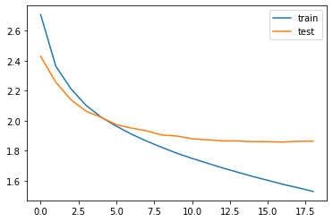
인퍼런스 모델 구현하기
테스트 단계에서 정수 인덱스 행렬로 존재하건 텍스트 데이터를 실제로 복원해야 하므로, 필요한 3개의 사전을 미리 준비
src_index_to_word = src_tokenizer.index_word # 원문 단어 집합에서 정수 -> 단어를 얻음
tar_word_to_index = tar_tokenizer.word_index # 요약 단어 집합에서 단어 -> 정수를 얻음
tar_index_to_word = tar_tokenizer.index_word # 요약 단어 집합에서 정수 -> 단어를 얻음
seq2seq는 훈련할 때와 실제 동작할 때(인퍼런스 단계)의 방식이 다르므로 그에 맞게 설계를 별개로 진행해야 한다.
# 인코더 설계
encoder_model = Model(inputs=encoder_inputs, outputs=[encoder_outputs, state_h, state_c])

# 이전 시점의 상태들을 저장하는 텐서
decoder_state_input_h = Input(shape=(hidden_size,))
decoder_state_input_c = Input(shape=(hidden_size,))

dec_emb2 = dec_emb_layer(decoder_inputs)

# 문장의 다음 단어를 예측하기 위해서 초기 상태(initial_state)를 이전 시점의 상태로 사용. 이는 뒤의 함수 decode_sequence()에 구현
# 훈련 과정에서와 달리 LSTM의 리턴하는 은닉 상태와 셀 상태인 state_h와 state_c를 버리지 않음.
decoder_outputs2, state_h2, state_c2 = decoder_lstm(dec_emb2, initial_state=[decoder_state_input_h, decoder_state_input_c])
# 어텐션 함수
decoder_hidden_state_input = Input(shape=(text_max_len, hidden_size))
attn_out_inf = attn_layer([decoder_outputs2, decoder_hidden_state_input])
decoder_inf_concat = Concatenate(axis=-1, name='concat')([decoder_outputs2, attn_out_inf])
# 디코더의 출력층
decoder_outputs2 = decoder_softmax_layer(decoder_inf_concat)
# 최종 디코더 모델
decoder_model = Model(
[decoder_inputs] + [decoder_hidden_state_input,decoder_state_input_h, decoder_state_input_c],
[decoder_outputs2] + [state_h2, state_c2])인퍼런스 단계에서 단어 시퀀스를 완성하는 함수
def decode_sequence(input_seq):
    # 입력으로부터 인코더의 상태를 얻음
    e_out, e_h, e_c = encoder_model.predict(input_seq)

     # <SOS>에 해당하는 토큰 생성
    target_seq = np.zeros((1,1))
    target_seq[0, 0] = tar_word_to_index['sostoken']

    stop_condition = False
    decoded_sentence = ''
    while not stop_condition: # stop_condition이 True가 될 때까지 루프 반복

        output_tokens, h, c = decoder_model.predict([target_seq] + [e_out, e_h, e_c])
        sampled_token_index = np.argmax(output_tokens[0, -1, :])
        sampled_token = tar_index_to_word[sampled_token_index]

        if (sampled_token!='eostoken'):
            decoded_sentence += ' '+sampled_token

        #  <eos>에 도달하거나 최대 길이를 넘으면 중단.
        if (sampled_token == 'eostoken'  or len(decoded_sentence.split()) >= (summary_max_len-1)):
            stop_condition = True

        # 길이가 1인 타겟 시퀀스를 업데이트
        target_seq = np.zeros((1,1))
        target_seq[0, 0] = sampled_token_index

        # 상태를 업데이트 합니다.
        e_h, e_c = h, c

    return decoded_sentence
모델 테스트하기
# 원문의 정수 시퀀스를 텍스트 시퀀스로 변환
def seq2text(input_seq):
    temp=''
    for i in input_seq:
        if (i!=0):
            temp = temp + src_index_to_word[i]+' '
    return temp

# 요약문의 정수 시퀀스를 텍스트 시퀀스로 변환
def seq2summary(input_seq):
    temp=''
    for i in input_seq:
        if ((i!=0 and i!=tar_word_to_index['sostoken']) and i!=tar_word_to_index['eostoken']):
            temp = temp + tar_index_to_word[i] + ' '
    return temp
for i in range(50, 100):
print("원문 :", seq2text(encoder_input_test[i]))
print("실제 요약 :", seq2summary(decoder_input_test[i]))
print("예측 요약 :", decode_sequence(encoder_input_test[i].reshape(1, text_max_len)))
print("\n")성능을 개선하는 방법
- seq2seq와 어텐션의 자체의 조합을 좀 더 좋게 수정
- 빔 서치(beam search)
- pre-trained word embedding
- 인코더-디코더 자체의 구조를 새로이 변경한 트랜스포머(Transformer)
추출적 요약 해보기
Summa 패키지에서 추출적 요약을 위한 summarize를 제공한다.
데이터 다운로드
import requests
from summa.summarizer import summarize

text = requests.get('http://rare-technologies.com/the_matrix_synopsis.txt').text
print(text[:1500])
'''
The screen is filled with green, cascading code which gives way to the title, The Matrix.

A phone rings and text appears on the screen: "Call trans opt: received. 2-19-98 13:24:18 REC: Log>" As a conversation takes place between Trinity (Carrie-Anne Moss) and Cypher (Joe Pantoliano), two free humans, a table of random green numbers are being scanned and individual numbers selected, creating a series of digits not unlike an ordinary phone number, as if a code is being deciphered or a call is being traced.

Trinity discusses some unknown person. Cypher taunts Trinity, suggesting she enjoys watching him. Trinity counters that "Morpheus (Laurence Fishburne) says he may be 'the One'," just as the sound of a number being selected alerts Trinity that someone may be tracing their call. She ends the call.

Armed policemen move down a darkened, decrepit hallway in the Heart O' the City Hotel, their flashlight beam bouncing just ahead of them. They come to room 303, kick down the door and find a woman dressed in black, facing away from them. It's Trinity. She brings her hands up from the laptop she's working on at their command.

Outside the hotel a car drives up and three agents appear in neatly pressed black suits. They are Agent Smith (Hugo Weaving), Agent Brown (Paul Goddard), and Agent Jones (Robert Taylor). Agent Smith and the presiding police lieutenant argue. Agent Smith admonishes the policeman that they were given specific orders to contact the agents first, for their
'''
summarize 사용하기
summarize의 인자
- text (str): 요약할 테스트.
- ratio (float, optional)– 요약문에서 원본에서 선택되는 문장 비율. 0~1 사이값
- words (int or None, optional) – 출력에 포함할 단어 수. 만약, ratio와 함께 두 파라미터가 모두 제공되는 경우 ratio는 무시한다.
- split (bool, optional) – True면 문장 list / False는 조인(join)된 문자열을 반환
Summa의 summarize는 문장 토큰화를 별도로 하지 않아도 내부적으로 문장 토큰화를 수행한다.
# ex
print('Summary:')
print(summarize(text, ratio=0.005))
'''
Summary:
Morpheus, Trinity, Neo, Apoc, Switch, Mouse and Cypher are jacked into the Matrix.
Trinity brings the helicopter down to the floor that Morpheus is on and Neo opens fire on the three Agents.
'''

# 출력을 리스트로 받기
print('Summary:')
print(summarize(text, ratio=0.005, split=True))
'''
Summary:
['Morpheus, Trinity, Neo, Apoc, Switch, Mouse and Cypher are jacked into the Matrix.', 'Trinity brings the helicopter down to the floor that Morpheus is on and Neo opens fire on the three Agents.']
'''

# 단어의 수로 요약문의 크기 조절
print('Summary:')
print(summarize(text, words=50))
'''
Summary:
Trinity takes Neo to Morpheus.
Morpheus, Trinity, Neo, Apoc, Switch, Mouse and Cypher are jacked into the Matrix.
Trinity brings the helicopter down to the floor that Morpheus is on and Neo opens fire on the three Agents.
''''AIFFEL > exploration' 카테고리의 다른 글
| Exploration 10 (0) | 2022.02.08 |
|---|---|
| Exploration 09 (0) | 2022.02.03 |
| Exploration 07 (0) | 2022.01.25 |
| Exploration 06 (0) | 2022.01.20 |
| Exploration 05 (0) | 2022.01.18 |