
Exploration 06
텍스트 감정분석의 유용성
오늘은 IMDb나 네이버 영화 리뷰 텍스트에 담긴 이용자의 감성이 긍정적인지 혹은 부정적인지를 분류(Classification)할 수 있는 딥러닝 모델을 만들어 볼 것이다.

Q&A
텍스트를 숫자로 표현하는 방법
텍스트의 중요한 특징은 그 자체로는 기호일 뿐이며, 텍스트가 내포하는 의미를 기호가 직접 내포하지 않는다는 것이다.
딥러닝을 통해 단어의 의미를 나타내는 벡터를 만들 수 있다.
i feel hungry
i eat lunch
now i feel happy
# 처리해야 할 문장을 파이썬 리스트에 옮겨 담았습니다.
sentences=['i feel hungry', 'i eat lunch', 'now i feel happy']

# 파이썬 split() 메소드를 이용해 단어 단위로 문장을 쪼개 봅니다.
word_list = 'i feel hungry'.split()

index_to_word={}  # 빈 딕셔너리를 만들어서

# 단어들을 하나씩 채워 봅니다. 채우는 순서는 일단 임의로 하였습니다. 그러나 사실 순서는 중요하지 않습니다.
# <BOS>, <PAD>, <UNK>는 관례적으로 딕셔너리 맨 앞에 넣어줍니다.
index_to_word[0]='<PAD>'  # 패딩용 단어
index_to_word[1]='<BOS>'  # 문장의 시작지점
index_to_word[2]='<UNK>'  # 사전에 없는(Unknown) 단어
index_to_word[3]='i'
index_to_word[4]='feel'
index_to_word[5]='hungry'
index_to_word[6]='eat'
index_to_word[7]='lunch'
index_to_word[8]='now'
index_to_word[9]='happy'

print(index_to_word)
'''
{0: '<PAD>', 1: '<BOS>', 2: '<UNK>', 3: 'i', 4: 'feel', 5: 'hungry', 6: 'eat', 7: 'lunch', 8: 'now', 9: 'happy'}
'''

# {텍스트:인덱스} 구조로 변경 (기존-> {인덱스:텍스트})
word_to_index={word:index for index, word in index_to_word.items()}
print(word_to_index)
'''
{'<PAD>': 0, '<BOS>': 1, '<UNK>': 2, 'i': 3, 'feel': 4, 'hungry': 5, 'eat': 6, 'lunch': 7, 'now': 8, 'happy': 9}
'''
이제 이 단어 사전에 단어를 입력하면 숫자로 바꿀 수 있다.
print(word_to_index['feel'])  # 단어 'feel'은 숫자 인덱스 4로 바뀝니다
# 4
함수화
- 한 문장을 숫자로 encode해준는 함수
- 여러 문장을 숫자로 encode해준는 함수
- 한 숫자 벡터를 문자로 decode 해주는 함수
- 여러 숫자 벡터를 문자로 decode 해주는 함수
# 문장 1개를 활용할 딕셔너리와 함께 주면, 단어 인덱스 리스트로 변환해 주는 함수를 만들어 봅시다.
# 단, 모든 문장은 <BOS>로 시작하는 것으로 합니다.
def get_encoded_sentence(sentence, word_to_index):
    return [word_to_index['<BOS>']]+[word_to_index[word] \
if word in word_to_index else word_to_index['<UNK>'] for word in sentence.split()]

print(get_encoded_sentence('i eat lunch', word_to_index))
'''
[1, 3, 6, 7]
'''

# 여러 개의 문장 리스트를 한꺼번에 숫자 텐서로 encode해 주는 함수입니다.
def get_encoded_sentences(sentences, word_to_index):
    return [get_encoded_sentence(sentence, word_to_index) for sentence in sentences]

# sentences=['i feel hungry', 'i eat lunch', 'now i feel happy'] 가 아래와 같이 변환됩니다.
encoded_sentences = get_encoded_sentences(sentences, word_to_index)
print(encoded_sentences)
'''
[[1, 3, 4, 5], [1, 3, 6, 7], [1, 8, 3, 4, 9]]
'''

# 숫자 벡터로 encode된 문장을 원래대로 decode하는 함수입니다.
def get_decoded_sentence(encoded_sentence, index_to_word):
    return ' '.join(index_to_word[index] if index in index_to_word else '<UNK>' for index in encoded_sentence[1:])  #[1:]를 통해 <BOS>를 제외

print(get_decoded_sentence([1, 3, 4, 5], index_to_word))
'''
i feel hungry
'''

# 여러 개의 숫자 벡터로 encode된 문장을 한꺼번에 원래대로 decode하는 함수입니다.
def get_decoded_sentences(encoded_sentences, index_to_word):
    return [get_decoded_sentence(encoded_sentence, index_to_word) for encoded_sentence in encoded_sentences]

# encoded_sentences=[[1, 3, 4, 5], [1, 3, 6, 7], [1, 8, 3, 4, 9]] 가 아래와 같이 변환됩니다.
print(get_decoded_sentences(encoded_sentences, index_to_word))
'''
['i feel hungry', 'i eat lunch', 'now i feel happy']
'''
Embedding 레이어의 등장
텍스트를 숫자로 변환하여 모델의 입력으로 사용될 수 있게 되었지만 이 벡터는 텍스트에 담긴 언어의 의미롸 대응되는 벡터가 아니라 임의로 부여된 단어의 순서에 불과하다. Tensorflow, Pytorch 등의 딥러닝 프레임워크들은 의미 벡터 파라미터를 구현한 Embedding 레이어를 제공한다.

‘great’는 먼저 1918이라는 index로 변환되고 lookup table에서 [1.2, 0.7, 1.9, 1.5]와 같은 Embedding vector로 변환된다.
# 아래 코드는 그대로 실행하시면 에러가 발생할 것입니다.

import numpy as np
import tensorflow as tf
import os

vocab_size = len(word_to_index)  # 위 예시에서 딕셔너리에 포함된 단어 개수는 10
word_vector_dim = 4    # 위 그림과 같이 4차원의 워드 벡터를 가정합니다.

embedding = tf.keras.layers.Embedding(input_dim=vocab_size, output_dim=word_vector_dim, mask_zero=True)

# 숫자로 변환된 텍스트 데이터 [[1, 3, 4, 5], [1, 3, 6, 7], [1, 8, 3, 4, 9]] 에 Embedding 레이어를 적용합니다.
raw_inputs = np.array(get_encoded_sentences(sentences, word_to_index), dtype='object')
output = embedding(raw_inputs)
print(output)
위의 코드는 에러를 발생하는 데 그 이유는 Embedding 레이어의 input이 되는 문장 벡터는 그 길이가 일정해야 하기 때문이다. (raw_input의 3개 벡터의 길이는 각각 4,4,5)
Tensorflow에서는 tf.keras.preprocessing.sequence.pad_sequences 라는 편리한 함수를 통해 문장 벡터 뒤에 패딩()을 추가하여 길이를 일정하게 맞춰주는 기능을 제공한다.
raw_inputs = tf.keras.preprocessing.sequence.pad_sequences(raw_inputs,
                                                       value=word_to_index['<PAD>'],
                                                       padding='post',
                                                       maxlen=5)
print(raw_inputs)
'''
[[1 3 4 5 0]
 [1 3 6 7 0]
 [1 8 3 4 9]]
'''
위의 코드 다시시도
vocab_size = len(word_to_index)  # 위 예시에서 딕셔너리에 포함된 단어 개수는 10
word_vector_dim = 4    # 그림과 같이 4차원의 워드 벡터를 가정합니다.

embedding = tf.keras.layers.Embedding(input_dim=vocab_size, output_dim=word_vector_dim, mask_zero=True)

# tf.keras.preprocessing.sequence.pad_sequences를 통해 word vector를 모두 일정 길이로 맞춰주어야
# embedding 레이어의 input이 될 수 있음에 주의해 주세요.
raw_inputs = np.array(get_encoded_sentences(sentences, word_to_index), dtype=object)
raw_inputs = tf.keras.preprocessing.sequence.pad_sequences(raw_inputs,
                                                       value=word_to_index['<PAD>'],
                                                       padding='post',
                                                       maxlen=5)
output = embedding(raw_inputs)
print(output)
'''
tf.Tensor(
[[[ 0.02096364  0.04570582  0.01623174 -0.03731489]
  [-0.00049068  0.03613648 -0.0483637  -0.01599956]
  [ 0.00528395  0.04702011  0.0020753  -0.01195306]
  [ 0.01520946 -0.02078022  0.04988812  0.02934435]
  [ 0.00972203  0.0051379   0.02984723 -0.01997231]]

 [[ 0.02096364  0.04570582  0.01623174 -0.03731489]
  [-0.00049068  0.03613648 -0.0483637  -0.01599956]
  [-0.04748726  0.04907146 -0.03113985  0.00511583]
  [ 0.01047821 -0.04604801  0.04600367 -0.04344996]
  [ 0.00972203  0.0051379   0.02984723 -0.01997231]]

 [[ 0.02096364  0.04570582  0.01623174 -0.03731489]
  [ 0.00446204  0.0051946   0.0275388   0.03405363]
  [-0.00049068  0.03613648 -0.0483637  -0.01599956]
  [ 0.00528395  0.04702011  0.0020753  -0.01195306]
  [ 0.04341961  0.00676854  0.01015236 -0.01791128]]], shape=(3, 5, 4), dtype=float32)
'''시퀀스 데이터를 다루는 RNN
주로 텍스트 데이터를 다루는 데 사용되는 Recurrent Neural Network(RNN) 은 시퀀스(Sequence) 형태의 데이터를 처리하기에 최적인 모델이다.
‘i feel hungry’라는 음성을 초당 한 단어씩, 3초에 걸쳐 음성 데이터로 이야기했을 때의 예를 보자.
at time=0s : 듣는이의 귀에 들어온 input='i'
at time=1s : 듣는이의 귀에 들어온 input='feel'
at time=2s : 듣는이의 귀에 들어온 input='hungry'
다음과 같이 입력이 시간의 축을 따라 발생하는 데이터가 시퀀스 데이터이다.
만약 times=1s인 시점에서 입력으로 받은 문자은 ‘i feel’까지이다. 그 다음에 어떠한 말이 올지는 알 수 없는 상황이다. RNN은 이런 상황을 묘사하기에 가장 적당한 모델 구조를 가지고 있다. 그 이유는 RNN은 시간의 흐름에 따라 새롭게 들어오는 입력에 따라 변하는 현재 상태를 묘사하는 state machine으로 설계되었기 때문이다.
state 예시

다음의 두 대화를 보면 Stateful 대화에서 직원은 손님이 이전에 주문한 내용을 기억하고 Stateless대화에서는 기억을 하지 못하고 있다.
김성훈 교수의 모두의 딥러닝 강좌 12강. RNN
- 현재의 state가 그 다음 state에 영향을 미친다.
- new state = f(old state, input)
- Vanilla RNN (기본적인 RNN)
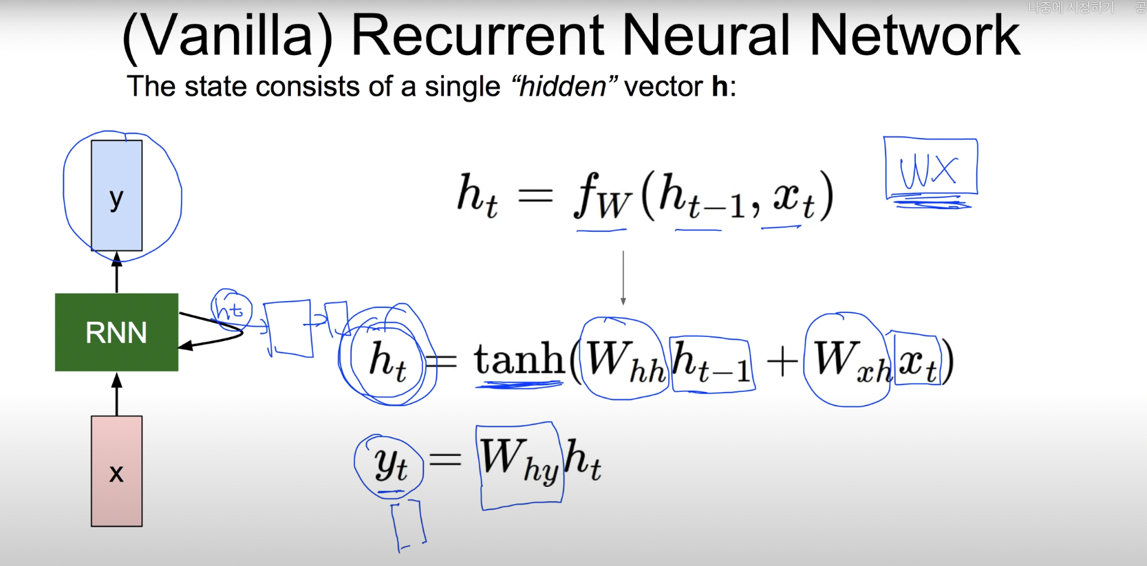
- weight값은 똑같은 것을 사용

- 알파벳이 주어 졌을 때 그 다음에 올 알파벳을 예측

- 각각의 알파벳을 원-핫 인코딩으로 변환 후
- 가중치를 곱한다. 이 때 전 layer에서 구하였던 h_score값의 영향을 받는다. (단. 첫 번째 layer는 전에 구한 layer의 h_score값이 없으므로 h_score을 0으로 두어 영향을 받지 않는다.)
- hidden layer이후에는 CNN과 같이 FC layer를 사용하여 score를 구한다.
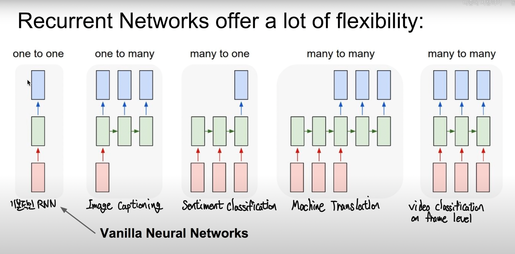
- RNN 활용 예시
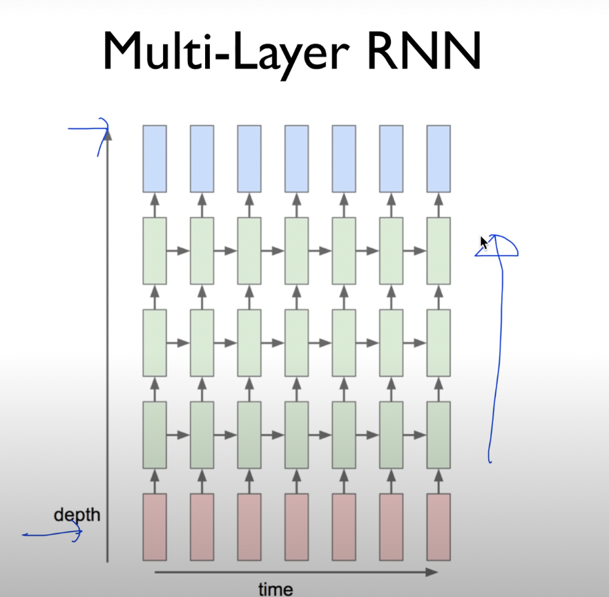
- RNN을 더 복잡한 layer를 사용하면 좋은 성능을 낼 수 있다.
Vanilla보다 몇 개의 더 좋은 모델
- Long Short Term Memory (LSTM)
- GRU
RNN 모델 구현 (LSTM)
vocab_size = 10  # 어휘 사전의 크기입니다(10개의 단어)
word_vector_dim = 4  # 단어 하나를 표현하는 임베딩 벡터의 차원수입니다.

model = tf.keras.Sequential()
model.add(tf.keras.layers.Embedding(vocab_size, word_vector_dim, input_shape=(None,)))
model.add(tf.keras.layers.LSTM(8))   # 가장 널리 쓰이는 RNN인 LSTM 레이어를 사용하였습니다. 이때 LSTM state 벡터의 차원수는 8로 하였습니다. (변경 가능)
model.add(tf.keras.layers.Dense(8, activation='relu'))
model.add(tf.keras.layers.Dense(1, activation='sigmoid'))  # 최종 출력은 긍정/부정을 나타내는 1dim 입니다.

model.summary()
'''
Model: "sequential"
_________________________________________________________________
Layer (type)                 Output Shape              Param #
=================================================================
embedding_3 (Embedding)      (None, None, 4)           40
_________________________________________________________________
lstm (LSTM)                  (None, 8)                 416
_________________________________________________________________
dense (Dense)                (None, 8)                 72
_________________________________________________________________
dense_1 (Dense)              (None, 1)                 9
=================================================================
Total params: 537
Trainable params: 537
Non-trainable params: 0
_________________________________________________________________
'''
꼭 RNN이어야 할까?
텍스트를 처리하기 위해 RNN이 아닌라 1-D Convolution Neural Network(1-D CNN) 를 사용할 수도 있다. 1-D CNN에서는 뭊아 전체를 한꺼번에 한 방향으로 길이 7짜리 피터로 스캐닝 하면서 7단어이내에서 발견되는 특징을 추출하여 그것으로 문장을 분류하는 방식을 사용한다.
특징
- RNN 못지않은 효율을 보여준다.
- CNN계열은 RNN계열보다 병열처리가 효율적이기 때문에 학습 속도도 훨씬 빠르다.
CNN 모델 구현 1
vocab_size = 10  # 어휘 사전의 크기입니다(10개의 단어)
word_vector_dim = 4   # 단어 하나를 표현하는 임베딩 벡터의 차원 수입니다.

model = tf.keras.Sequential()
model.add(tf.keras.layers.Embedding(vocab_size, word_vector_dim, input_shape=(None,)))
model.add(tf.keras.layers.Conv1D(16, 7, activation='relu'))
model.add(tf.keras.layers.MaxPooling1D(5))
model.add(tf.keras.layers.Conv1D(16, 7, activation='relu'))
model.add(tf.keras.layers.GlobalMaxPooling1D())
model.add(tf.keras.layers.Dense(8, activation='relu'))
model.add(tf.keras.layers.Dense(1, activation='sigmoid'))  # 최종 출력은 긍정/부정을 나타내는 1dim 입니다.

model.summary()
'''
Model: "sequential_1"
_________________________________________________________________
Layer (type)                 Output Shape              Param #
=================================================================
embedding_4 (Embedding)      (None, None, 4)           40
_________________________________________________________________
conv1d (Conv1D)              (None, None, 16)          464
_________________________________________________________________
max_pooling1d (MaxPooling1D) (None, None, 16)          0
_________________________________________________________________
conv1d_1 (Conv1D)            (None, None, 16)          1808
_________________________________________________________________
global_max_pooling1d (Global (None, 16)                0
_________________________________________________________________
dense_2 (Dense)              (None, 8)                 136
_________________________________________________________________
dense_3 (Dense)              (None, 1)                 9
=================================================================
Total params: 2,457
Trainable params: 2,457
Non-trainable params: 0
_________________________________________________________________
'''
CNN 모델 구현 2
vocab_size = 10  # 어휘 사전의 크기입니다(10개의 단어)
word_vector_dim = 4   # 단어 하나를 표현하는 임베딩 벡터의 차원 수입니다.

model = tf.keras.Sequential()
model.add(tf.keras.layers.Embedding(vocab_size, word_vector_dim, input_shape=(None,)))
model.add(tf.keras.layers.GlobalMaxPooling1D())
model.add(tf.keras.layers.Dense(8, activation='relu'))
model.add(tf.keras.layers.Dense(1, activation='sigmoid'))  # 최종 출력은 긍정/부정을 나타내는 1dim 입니다.

model.summary()
'''
Model: "sequential_2"
_________________________________________________________________
Layer (type)                 Output Shape              Param #
=================================================================
embedding_5 (Embedding)      (None, None, 4)           40
_________________________________________________________________
global_max_pooling1d_1 (Glob (None, 4)                 0
_________________________________________________________________
dense_4 (Dense)              (None, 8)                 40
_________________________________________________________________
dense_5 (Dense)              (None, 1)                 9
=================================================================
Total params: 89
Trainable params: 89
Non-trainable params: 0
'''
다른 방법
- 1-D CNN과 RNN을 섞어 사용
- FFN(FeedForwaed Network)
- Transformer 사용
IMDB 영화리뷰 감성분석
IMDB 데이터셋 분석
IMDb Large Movie Dataset
- 50000개의 영어로 작성된 영화 리뷰 텍스트 (train: 25000, test: 25000)
- 긍정은 1, 부정은 0의 라벨
데이터 확인
imdb = tf.keras.datasets.imdb

# IMDb 데이터셋 다운로드
(x_train, y_train), (x_test, y_test) = imdb.load_data(num_words=10000)
print("훈련 샘플 개수: {}, 테스트 개수: {}".format(len(x_train), len(x_test)))
'''
훈련 샘플 개수: 25000, 테스트 개수: 25000
'''
# 숫자로 encode된 텍스트 데이터
print(x_train[0]) # 1번째 리뷰데이터
print('라벨: ', y_train[0]) # 1번째 리뷰데이터의 라벨
print('1번째 리뷰 문장 길이: ', len(x_train[0]))
print('2번째 리뷰 문장 길이: ', len(x_train[1]))
'''
[1, 14, 22, 16, 43, 530, 973, 1622, 1385, 65, 458, 4468, 66, 3941, 4, 173, 36, 256, 5, 25, 100, 43, 838, 112, 50, 670, 2, 9, 35, 480, 284, 5, 150, 4, 172, 112, 167, 2, 336, 385, 39, 4, 172, 4536, 1111, 17, 546, 38, 13, 447, 4, 192, 50, 16, 6, 147, 2025, 19, 14, 22, 4, 1920, 4613, 469, 4, 22, 71, 87, 12, 16, 43, 530, 38, 76, 15, 13, 1247, 4, 22, 17, 515, 17, 12, 16, 626, 18, 2, 5, 62, 386, 12, 8, 316, 8, 106, 5, 4, 2223, 5244, 16, 480, 66, 3785, 33, 4, 130, 12, 16, 38, 619, 5, 25, 124, 51, 36, 135, 48, 25, 1415, 33, 6, 22, 12, 215, 28, 77, 52, 5, 14, 407, 16, 82, 2, 8, 4, 107, 117, 5952, 15, 256, 4, 2, 7, 3766, 5, 723, 36, 71, 43, 530, 476, 26, 400, 317, 46, 7, 4, 2, 1029, 13, 104, 88, 4, 381, 15, 297, 98, 32, 2071, 56, 26, 141, 6, 194, 7486, 18, 4, 226, 22, 21, 134, 476, 26, 480, 5, 144, 30, 5535, 18, 51, 36, 28, 224, 92, 25, 104, 4, 226, 65, 16, 38, 1334, 88, 12, 16, 283, 5, 16, 4472, 113, 103, 32, 15, 16, 5345, 19, 178, 32]
라벨: 1
1번째 리뷰 문장 길이: 218
2번째 리뷰 문장 길이: 189
'''# encode에 사용한 딕셔너리
word_to_index = imdb.get_word_index()
index_to_word = {index:word for word, index in word_to_index.items()}
print(index_to_word[1]) # 'the' 가 출력됩니다.
print(word_to_index['the']) # 1 이 출력됩니다.
'''
the
1
'''# 실제로는 3개씩 인덱스가 밀려있어서 앞에 3개를 추가하여 인덱스 맞추기
#실제 인코딩 인덱스는 제공된 word_to_index에서 index 기준으로 3씩 뒤로 밀려 있습니다.
word_to_index = {k:(v+3) for k,v in word_to_index.items()}
# 처음 몇 개 인덱스는 사전에 정의되어 있습니다
word_to_index["<PAD>"] = 0
word_to_index["<BOS>"] = 1
word_to_index["<UNK>"] = 2 # unknown
word_to_index["<UNUSED>"] = 3
index_to_word = {index:word for word, index in word_to_index.items()}
print(index_to_word[1]) # '<BOS>' 가 출력됩니다.
print(word_to_index['the']) # 4 이 출력됩니다.
print(index_to_word[4]) # 'the' 가 출력됩니다.
'''
<BOS>
4
the
'''# decode동작 확인
print(get_decoded_sentence(x_train[0], index_to_word))
print('라벨: ', y_train[0]) # 1번째 리뷰데이터의 라벨
'''
this film was just brilliant casting location scenery story direction everyone's really suited the part they played and you could just imagine being there robert <UNK> is an amazing actor and now the same being director <UNK> father came from the same scottish island as myself so i loved the fact there was a real connection with this film the witty remarks throughout the film were great it was just brilliant so much that i bought the film as soon as it was released for <UNK> and would recommend it to everyone to watch and the fly fishing was amazing really cried at the end it was so sad and you know what they say if you cry at a film it must have been good and this definitely was also <UNK> to the two little boy's that played the <UNK> of norman and paul they were just brilliant children are often left out of the <UNK> list i think because the stars that play them all grown up are such a big profile for the whole film but these children are amazing and should be praised for what they have done don't you think the whole story was so lovely because it was true and was someone's life after all that was shared with us all
라벨: 1
'''total_data_text = list(x_train) + list(x_test)
# 텍스트데이터 문장길이의 리스트를 생성한 후
num_tokens = [len(tokens) for tokens in total_data_text]
num_tokens = np.array(num_tokens)
# 문장길이의 평균값, 최대값, 표준편차를 계산해 본다.
print('문장길이 평균 : ', np.mean(num_tokens))
print('문장길이 최대 : ', np.max(num_tokens))
print('문장길이 표준편차 : ', np.std(num_tokens))
# 예를들어, 최대 길이를 (평균 + 2*표준편차)로 한다면,
max_tokens = np.mean(num_tokens) + 2 * np.std(num_tokens)
maxlen = int(max_tokens)
print('pad_sequences maxlen : ', maxlen)
print('전체 문장의 {}%가 maxlen 설정값 이내에 포함됩니다. '.format(np.sum(num_tokens < max_tokens) / len(num_tokens)))
'''
문장길이 평균 : 234.75892
문장길이 최대 : 2494
문장길이 표준편차 : 172.91149458735703
pad_sequences maxlen : 580
전체 문장의 0.94536%가 maxlen 설정값 이내에 포함됩니다.
'''train, test 데이터 생성
# padding 방식 결정
x_train = tf.keras.preprocessing.sequence.pad_sequences(x_train,
                                                        value=word_to_index["<PAD>"],
                                                        padding='post', # 혹은 'pre'
                                                        maxlen=maxlen)

x_test = tf.keras.preprocessing.sequence.pad_sequences(x_test,
                                                       value=word_to_index["<PAD>"],
                                                       padding='post', # 혹은 'pre'
                                                       maxlen=maxlen)

print(x_train.shape)
'''
(25000, 580)
'''모델 설계
vocab_size = 10000    # 어휘 사전의 크기입니다(10,000개의 단어)
word_vector_dim = 16  # 워드 벡터의 차원 수 (변경 가능한 하이퍼파라미터)

# model 설계 - 딥러닝 모델 코드를 직접 작성해 주세요.
model = tf.keras.Sequential()
# [[YOUR CODE]]
model.add(tf.keras.layers.Embedding(vocab_size, word_vector_dim, input_shape=(None,)))
model.add(tf.keras.layers.LSTM(8))   # 가장 널리 쓰이는 RNN인 LSTM 레이어를 사용하였습니다. 이때 LSTM state 벡터의 차원수는 8로 하였습니다. (변경 가능)
model.add(tf.keras.layers.Dense(8, activation='relu'))
model.add(tf.keras.layers.Dense(1, activation='sigmoid'))

model.summary()
'''
Model: "sequential_4"
_________________________________________________________________
Layer (type)                 Output Shape              Param #
=================================================================
embedding_6 (Embedding)      (None, None, 16)          160000
_________________________________________________________________
lstm_1 (LSTM)                (None, 8)                 800
_________________________________________________________________
dense_6 (Dense)              (None, 8)                 72
_________________________________________________________________
dense_7 (Dense)              (None, 1)                 9
=================================================================
Total params: 160,881
Trainable params: 160,881
Non-trainable params: 0
_________________________________________________________________
'''
validation set 분리
# validation set 10000건 분리
x_val = x_train[:10000]
y_val = y_train[:10000]

# validation set을 제외한 나머지 15000건
partial_x_train = x_train[10000:]
partial_y_train = y_train[10000:]

print(partial_x_train.shape)
print(partial_y_train.shape)
'''
(15000, 580)
(15000,)
'''
모델 학습
model.compile(optimizer='adam',
              loss='binary_crossentropy',
              metrics=['accuracy'])

epochs=20  # 몇 epoch를 훈련하면 좋을지 결과를 보면서 바꾸어 봅시다.

history = model.fit(partial_x_train,
                    partial_y_train,
                    epochs=epochs,
                    batch_size=512,
                    validation_data=(x_val, y_val),
                    verbose=1)
'''
loss: 0.6897 - accuracy: 0.5261 - val_loss: 0.6937 - val_accuracy: 0.5048
'''
모델 평가
results = model.evaluate(x_test,  y_test, verbose=2)

print(results)
'''
782/782 - 5s - loss: 0.6933 - accuracy: 0.5075
[0.6932967901229858, 0.5074800252914429]
'''
평가 시각화
history_dict = history.history
print(history_dict.keys()) # epoch에 따른 그래프를 그려볼 수 있는 항목들
'''
dict_keys(['loss', 'accuracy', 'val_loss', 'val_accuracy'])
'''

import matplotlib.pyplot as plt

acc = history_dict['accuracy']
val_acc = history_dict['val_accuracy']
loss = history_dict['loss']
val_loss = history_dict['val_loss']

epochs = range(1, len(acc) + 1)

# "bo"는 "파란색 점"입니다
plt.plot(epochs, loss, 'bo', label='Training loss')
# b는 "파란 실선"입니다
plt.plot(epochs, val_loss, 'b', label='Validation loss')
plt.title('Training and validation loss')
plt.xlabel('Epochs')
plt.ylabel('Loss')
plt.legend()

plt.show()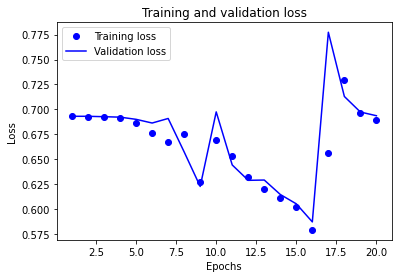
plt.clf()   # 그림을 초기화합니다

plt.plot(epochs, acc, 'bo', label='Training acc')
plt.plot(epochs, val_acc, 'b', label='Validation acc')
plt.title('Training and validation accuracy')
plt.xlabel('Epochs')
plt.ylabel('Accuracy')
plt.legend()

plt.show()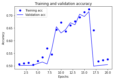
Word Embedding
💡 워드 임베딩(word embedding)
라벨링 비용이 많이 드는 머신러닝 기반 감성분석의 비용을 절감하면서 정확도를 크게 향상시킬 수 있는 자연어처리 기법 (단어의 특성을 저차원 벡터값으로 표현할 수 있음)
지금까지 사용한 Embedding 레이어
- (우리가 가진 사전의 단어 개수) x (워드 벡터 사이즈)만큼의 크기
# Embedding layer의 학습된 wordvector 확인
embedding_layer = model.layers[0]
weights = embedding_layer.get_weights()[0]
print(weights.shape)    # shape: (vocab_size, embedding_dim)
'''
(10000, 16)
'''
# 학습한 Embedding 파라미터를 파일에 써서 저장합니다.
word2vec_file_path = os.getenv('HOME')+'/aiffel/sentiment_classification/data/word2vec.txt'
f = open(word2vec_file_path, 'w')
f.write('{} {}\n'.format(vocab_size-4, word_vector_dim)) # 몇개의 벡터를 얼마 사이즈로 기재할지 타이틀을 씁니다.
# 단어 개수(에서 특수문자 4개는 제외하고)만큼의 워드 벡터를 파일에 기록합니다.
vectors = model.get_weights()[0]
for i in range(4,vocab_size):
f.write('{} {}\n'.format(index_to_word[i], ' '.join(map(str, list(vectors[i, :])))))
f.close()gensim package
gensim패키지로 저장한 임베딩 파라미터를 읽어서 wordvector로 사용
from gensim.models.keyedvectors import Word2VecKeyedVectors

word_vectors = Word2VecKeyedVectors.load_word2vec_format(word2vec_file_path, binary=False)
vector = word_vectors['computer']
vector
'''
array([-0.05156684, -0.05027233,  0.03619769, -0.00985204,  0.01735285,
        0.02981805,  0.0511942 , -0.01146023, -0.01958035, -0.00826631,
        0.02113515,  0.00083194,  0.03631599,  0.00501615,  0.04324353,
       -0.00967919], dtype=float32)
'''
gensim를 이용하여 특정 단어와 가장 유사한 단어, 유사도 확인
word_vectors.similar_by_word("love")
'''
[('exceptional', 0.9821829795837402),
 ('step', 0.9752857089042664),
 ('easier', 0.9750139117240906),
 ('heath', 0.9734551310539246),
 ('solid', 0.9727447628974915),
 ('revealed', 0.9727013111114502),
 ('halloween', 0.97214674949646),
 ('futuristic', 0.9710436463356018),
 ('9', 0.9704533815383911),
 ('terrific', 0.9700677394866943)]
'''
우리가 다룬 정도의 훈련 데이터로는 워드 벡터를 정교하게 학습시키기 어렵다.
Word2Vec 사용
- google세어 제공하는 사전학습된 워드 임베딩 모델
- 1억 개의 단어로 구성된 Google News dataset을 바탕으로 학습
- 총 300만 개의 단어를 각각 300차원의 벡터로 표현
# 300만개 중 100만개만 로딩

from gensim.models import KeyedVectors

word2vec_path = os.getenv('HOME')+'/aiffel/sentiment_classification/data/GoogleNews-vectors-negative300.bin.gz'
word2vec = KeyedVectors.load_word2vec_format(word2vec_path, binary=True, limit=1000000)
vector = word2vec['computer']
vector     # 무려 300dim의 워드 벡터입니다.
Word2Vec를 가지고 유사도 확인
# 메모리를 다소 많이 소비하는 작업이니 유의해 주세요.
word2vec.similar_by_word("love")
'''
[('loved', 0.6907791495323181),
 ('adore', 0.6816873550415039),
 ('loves', 0.661863386631012),
 ('passion', 0.6100708842277527),
 ('hate', 0.600395679473877),
 ('loving', 0.5886635780334473),
 ('Ilove', 0.5702950954437256),
 ('affection', 0.5664337873458862),
 ('undying_love', 0.5547304749488831),
 ('absolutely_adore', 0.5536840558052063)]
'''
학습했던 모델의 임베딩 레이어를 Word2Vec의 것으로 교체하여 다시 학습
vocab_size = 10000    # 어휘 사전의 크기입니다(10,000개의 단어)
word_vector_dim = 300  # 워드 벡터의 차원수
embedding_matrix = np.random.rand(vocab_size, word_vector_dim)

# embedding_matrix에 Word2Vec 워드 벡터를 단어 하나씩마다 차례차례 카피한다.
for i in range(4,vocab_size):
    if index_to_word[i] in word2vec:
        embedding_matrix[i] = word2vec[index_to_word[i]]
from tensorflow.keras.initializers import Constant
vocab_size = 10000 # 어휘 사전의 크기입니다(10,000개의 단어)
word_vector_dim = 300 # 워드 벡터의 차원 수
# 모델 구성
model = tf.keras.Sequential()
model.add(tf.keras.layers.Embedding(vocab_size,
word_vector_dim,
embeddings_initializer=Constant(embedding_matrix), # 카피한 임베딩을 여기서 활용
input_length=maxlen,
trainable=True)) # trainable을 True로 주면 Fine-tuning
model.add(tf.keras.layers.Conv1D(16, 7, activation='relu'))
model.add(tf.keras.layers.MaxPooling1D(5))
model.add(tf.keras.layers.Conv1D(16, 7, activation='relu'))
model.add(tf.keras.layers.GlobalMaxPooling1D())
model.add(tf.keras.layers.Dense(8, activation='relu'))
model.add(tf.keras.layers.Dense(1, activation='sigmoid'))
model.summary()
'''
Model: "sequential_5"
_________________________________________________________________
Layer (type) Output Shape Param #
=================================================================
embedding_7 (Embedding) (None, 580, 300) 3000000
_________________________________________________________________
conv1d_2 (Conv1D) (None, 574, 16) 33616
_________________________________________________________________
max_pooling1d_1 (MaxPooling1 (None, 114, 16) 0
_________________________________________________________________
conv1d_3 (Conv1D) (None, 108, 16) 1808
_________________________________________________________________
global_max_pooling1d_2 (Glob (None, 16) 0
_________________________________________________________________
dense_8 (Dense) (None, 8) 136
_________________________________________________________________
dense_9 (Dense) (None, 1) 9
=================================================================
Total params: 3,035,569
Trainable params: 3,035,569
Non-trainable params: 0
_________________________________________________________________
'''학습
# 학습의 진행
model.compile(optimizer='adam',
              loss='binary_crossentropy',
              metrics=['accuracy'])

epochs=20  # 몇 epoch를 훈련하면 좋을지 결과를 보면서 바꾸어 봅시다.

history = model.fit(partial_x_train,
                    partial_y_train,
                    epochs=epochs,
                    batch_size=512,
                    validation_data=(x_val, y_val),
                    verbose=1)
평가
# 테스트셋을 통한 모델 평가
results = model.evaluate(x_test,  y_test, verbose=2)

print(results)
'''
782/782 - 2s - loss: 0.5900 - accuracy: 0.8573
[0.5900180339813232, 0.8572800159454346]
''''AIFFEL > exploration' 카테고리의 다른 글
| Exploration 08 (0) | 2022.01.27 |
|---|---|
| Exploration 07 (0) | 2022.01.25 |
| Exploration 05 (0) | 2022.01.18 |
| Exploration 04 (0) | 2022.01.13 |
| Exploration 03 (0) | 2022.01.11 |