
Fundamental 23
딥러닝은 y = Wx + by=Wx+b 에서 최적의 WW(Weight)과 b를 찾는 과정이다. 이러한 과정을 딥러닝의 미싱 링크라고 한다.
데이터에서 원하는 특징을 효과적으로 추출하기 위해선 올바른 Weight를 정의하는 과정이 중요하다.
데이터의 형태
딥러닝을 이해하는 방법 중 가장 쉬운 방법은 데이터의 형태 변화를 쫓는 것이다.
이미지 데이터는 보통 채널(Channel)이라는 것을 가진다. 우리가 일상적으로 사용하는 것은 대부분 RGB 이미지이다.
레이어는 어렵다?
레이어(layer)란?
하나의 물체가 여러 개의 논리적인 객체들로 구성되어 있는 경우, 이러한 각각의 객체를 하나의 레이어라고 한다.
딥러닝의 근본! Linear 레이어
Fully Connected Layer, Feedforward Neural Network, Multilayer Perceptrons, Dense Layer... 등 다양한 이름으로 불리지만 그 모든 것들은 결국 Linear 레이어에 해당된다.
가중치 (Weight)
Linear layer는 선형 변환을 활용해 데이터를 특정 차원으로 변환하는 기능을 한다.
ex) 100차원의 데이터를 300차원으로 변환한다면 데이터를 더 풍부하게 표현한느 효과가 있고, 반대로 10차원의 데이터롤 변환한다면 데이터를 집약시키는 효과가 있다.
Linear layer는 (입력의 차원, 출력의 차원)에 해당하는 Weight를 가지는 특성을 가지고 있다.
데이터 집약
<식1>
1단계: (4, 2) x (2, 1) 행렬 = (4, )
2단계: (4, ) x (4, 1) 행렬 = (1, )
import tensorflow as tf

batch_size = 64
boxes = tf.zeros((batch_size, 4, 2))     # Tensorflow는 Batch를 기반으로 동작하기에,
                                         # 우리는 사각형 2개 세트를 batch_size개만큼
                                         # 만든 후 처리를 하게 됩니다.
print("1단계 연산 준비:", boxes.shape)

first_linear = tf.keras.layers.Dense(units=1, use_bias=False)
# units은 출력 차원 수를 의미합니다.
# Weight 행렬 속 실수를 인간의 뇌 속 하나의 뉴런 '유닛' 취급을 하는 거죠!

first_out = first_linear(boxes)
first_out = tf.squeeze(first_out, axis=-1) # (4, 1)을 (4,)로 변환해줍니다.
                                           # (불필요한 차원 축소)

print("1단계 연산 결과:", first_out.shape)
print("1단계 Linear Layer의 Weight 형태:", first_linear.weights[0].shape)

print("\n2단계 연산 준비:", first_out.shape)

second_linear = tf.keras.layers.Dense(units=1, use_bias=False)
second_out = second_linear(first_out)
second_out = tf.squeeze(second_out, axis=-1)

print("2단계 연산 결과:", second_out.shape)
print("2단계 Linear Layer의 Weight 형태:", second_linear.weights[0].shape)
'''
1단계 연산 준비: (64, 4, 2)
1단계 연산 결과: (64, 4)
1단계 Linear Layer의 Weight 형태: (2, 1)

2단계 연산 준비: (64, 4)
2단계 연산 결과: (64,)
2단계 Linear Layer의 Weight 형태: (4, 1)
'''
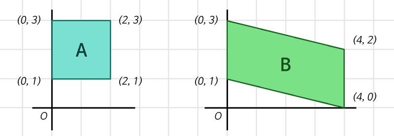
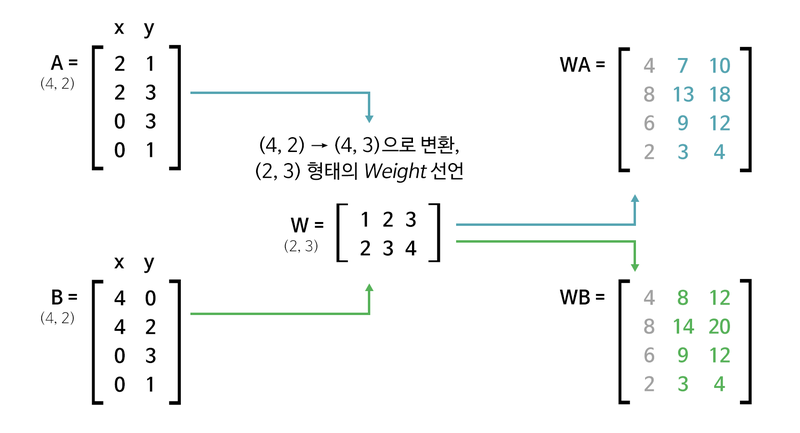
다른 행렬식 두 개(A,B)가 가중치(W)를 지나니 값이 똑같아 졌다. 이는 총 6개(위 그림에서는 2개)의 paramerter로 이문제를 해결하기엔 역부족하다는 것을 의미한다.
데이터 풍부
<식2>
1단계: (4, 2) x (2 x 3) 행렬 = (4, 3)
2단계: (4, 3) x (3 x 1) 행렬 = (4, )
3단계: (4, ) x (4 x 1) 행렬 = (1, )
1단계의 결과로 각 사각형에 대해 독립적인 정보가 생겨나기 시작한다. 이는 첫 번째 접근에 비해 더 많은 사각형을 구분해낼 수 있다.
import tensorflow as tf

batch_size = 64
boxes = tf.zeros((batch_size, 4, 2))

print("1단계 연산 준비:", boxes.shape)

first_linear = tf.keras.layers.Dense(units=3, use_bias=False)
first_out = first_linear(boxes)

print("1단계 연산 결과:", first_out.shape)
print("1단계 Linear Layer의 Weight 형태:", first_linear.weights[0].shape)

print("\n2단계 연산 준비:", first_out.shape)

second_linear = tf.keras.layers.Dense(units=1, use_bias=False)
second_out = second_linear(first_out)
second_out = tf.squeeze(second_out, axis=-1)

print("2단계 연산 결과:", second_out.shape)
print("2단계 Linear Layer의 Weight 형태:", second_linear.weights[0].shape)

print("\n3단계 연산 준비:", second_out.shape)

third_linear = tf.keras.layers.Dense(units=1, use_bias=False)
third_out = third_linear(second_out)
third_out = tf.squeeze(third_out, axis=-1)

print("3단계 연산 결과:", third_out.shape)
print("3단계 Linear Layer의 Weight 형태:", third_linear.weights[0].shape)

total_params = \
first_linear.count_params() + \
second_linear.count_params() + \
third_linear.count_params()

print("총 Parameters:", total_params)
'''
1단계 연산 준비: (64, 4, 2)
1단계 연산 결과: (64, 4, 3)
1단계 Linear Layer의 Weight 형태: (2, 3)

2단계 연산 준비: (64, 4, 3)
2단계 연산 결과: (64, 4)
2단계 Linear Layer의 Weight 형태: (3, 1)

3단계 연산 준비: (64, 4)
3단계 연산 결과: (64,)
3단계 Linear Layer의 Weight 형태: (4, 1)
총 Parameters: 13
'''- Parameter가 지나치게 많은 것은 Overfitting을 야기하기 때문에 Parameter가 많다고 무작정 좋은 것은 아니다.
편향 (Bias)
인사라는 행위를 y= wx라고 한다면 우리나라 인사법을 y =wx + 유교사상, 프랑스의 인사법을 y = wx + 아메리칸 마인드라고 표현할 수 있다.

- 원점을 평행이동하는 것만으로도 해결할 수 있기 때문에 실제로 편향은 선형변환된 값에 편향 파라미터 b를 더해주는 것으로 표현한다.
정보를 집약시키자! Comvolution 레이어
<식3>
1단계: (1920, 1080, 3) → (1920 x 1080 x 3, )
2단계: (6220800, ) x [6220800 x 1 Weight] = (1, )
<식 3>에 따르면 아무리 적어도 620만 개의 Parameter가 생성된다. 그래서 고안된 것이 Convolution layer이다.
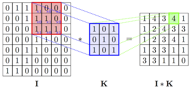

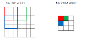
- filter: 커널이라고 불리는 Conv연산과정의 변수값
- Stride: filter가 움직이는 step
- Padding: Conv연산이 입력의 형태를 변형시키기 때문에 이를 방지하기 위해 사용

단 하나의 필터가 아닌 수십 개의 필터를 중첩해서 사용한다.
<식 4>
1단계: (1920, 1080, 3) x [3 x 16 x 5 x 5 Weight & Stride 5] = (384, 216, 16)
2단계: (384, 216, 16) → (384 x 216 x 16, )
3단계: (1327104, ) x [1327104 x 1 Weight] = (1, )
import tensorflow as tf

batch_size = 64
pic = tf.zeros((batch_size, 1920, 1080, 3))

print("입력 이미지 데이터:", pic.shape)
conv_layer = tf.keras.layers.Conv2D(filters=16,
                                    kernel_size=(5, 5),
                                    strides=5,
                                    use_bias=False)
conv_out = conv_layer(pic)

print("\nConvolution 결과:", conv_out.shape)
print("Convolution Layer의 Parameter 수:", conv_layer.count_params())

flatten_out = tf.keras.layers.Flatten()(conv_out)
print("\n1차원으로 펼친 데이터:", flatten_out.shape)

linear_layer = tf.keras.layers.Dense(units=1, use_bias=False)
linear_out = linear_layer(flatten_out)

print("\nLinear 결과:", linear_out.shape)
print("Linear Layer의 Parameter 수:", linear_layer.count_params())
'''
입력 이미지 데이터: (64, 1920, 1080, 3)

Convolution 결과: (64, 384, 216, 16)
Convolution Layer의 Parameter 수: 1200

1차원으로 펼친 데이터: (64, 1327104)

Linear 결과: (64, 1)
Linear Layer의 Parameter 수: 1327104
'''
핵심만 추려서 더 넓게! Pooling 레이어
Receptive Field 개념
Receptive Field란?
Receptive Field란 수용영역이며 Neural Network의 출력부가 충분한 정보를 얻기 위해 커버하는 입력 데이터의 Receptive Field가 충분히 커서 그 안에 detect해야 할 object의 특성이 충분히 포함되어 있어야 정확한 detection이 가능하게 된다.
Pooling
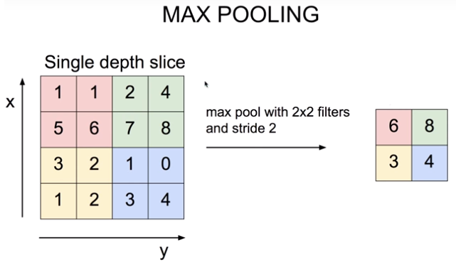
Max Pooling 레이어의 의미
효과
- translational invariance 효과: 이미지는 약간의 상하좌우 시프트가 생긴다고 해도 내용상 동일한 특징이 있는데, Max Pooling을 통해 인접한 영역 중 가장 특징이 두드러진 영역 하나를 뽑는 것은 오히려 약간의 시프트 효과에도 불구하고 동일한 특징을 안정적으로 잡아낼 수 있는 긍정적 효과가 있어서 오히려 object 위치에 대한 오버피팅을 방지하고 안정적인 특징 추출 효과를 가져온다.
- Non-linear 함수와 동일한 피처 추출 효과: Relu와 같은 Non-linear 함수도 마찬가지로 많은 하위 레이어의 연산 결과를 무시하는 효과를 발생시키지만, 그 결과 중요한 피처만을 상위 레이어로 추출해서 올려줌으로써 결과적으로 분류기의 성능을 증진시키는 효과를 가집니다. Min/Max Pooling도 이와 동일한 효과를 가지게 된다.
- Receptive Field 극대화 효과: Max Pooling이 없이도 Receptive Field를 크게 하려면 Convolutional 레이어를 아주 많이 쌓아야 한다. 그 결과 큰 파라미터 사이즈로 인한 오버피팅, 연산량 증가, Gradient Vanishing 등의 문제를 감수해야 합니다. 이런 문제를 효과적으로 해결하는 방법으로 꼽히는 두 가지 중 하나가 Max Pooling 레이어 사용입니다. 다른 하나로는 Dilated Convolution이 있습니다.
집약된 정보의 복원! Deconvolution 레이어
Conv layer는 데이터를 집약시키기 때문에 원본 데이터의 정보를 너무 많이 손실시킨것이 아닐까?
그래서 Conv의 결과를 역재생해서 원본 이미지와 최대한 유사한 정보를 복원해 내는 Auto Encoder라는 것이있다.
패키지 임포트 및 MNIST 데이터셋 로딩
import numpy as np
from tensorflow.keras.layers import Input, Dense, Conv2D, MaxPooling2D, UpSampling2D
from tensorflow.keras.models import Model
from tensorflow.keras.datasets import mnist
import json
import matplotlib.pyplot as plt #for plotting

# MNIST 데이터 로딩
(x_train, _), (x_test, _) = mnist.load_data()    # y_train, y_test는 사용하지 않습니다.

x_train = np.expand_dims(x_train, axis=3)
x_test = np.expand_dims(x_test, axis=3)

x_train = x_train.astype('float32') / 255.
x_test = x_test.astype('float32') / 255.- Auto Encoder의 라벨은 자기 자신이다.
AutoEncoder 모델 구성
# AutoEncoder 모델 구성 - Input 부분
input_shape = x_train.shape[1:]
input_img = Input(shape=input_shape)

# AutoEncoder 모델 구성 - Encoder 부분
encode_conv_layer_1 = Conv2D(16, (3, 3), activation='relu', padding='same')
encode_pool_layer_1 = MaxPooling2D((2, 2), padding='same')
encode_conv_layer_2 = Conv2D(8, (3, 3), activation='relu', padding='same')
encode_pool_layer_2 = MaxPooling2D((2, 2), padding='same')
encode_conv_layer_3 = Conv2D(4, (3, 3), activation='relu', padding='same')
encode_pool_layer_3 = MaxPooling2D((2, 2), padding='same')

encoded = encode_conv_layer_1(input_img)
encoded = encode_pool_layer_1(encoded)
encoded = encode_conv_layer_2(encoded)
encoded = encode_pool_layer_2(encoded)
encoded = encode_conv_layer_3(encoded)
encoded = encode_pool_layer_3(encoded)

# AutoEncoder 모델 구성 - Decoder 부분
decode_conv_layer_1 = Conv2D(4, (3, 3), activation='relu', padding='same')
decode_upsample_layer_1 = UpSampling2D((2, 2))
decode_conv_layer_2 = Conv2D(8, (3, 3), activation='relu', padding='same')
decode_upsample_layer_2 = UpSampling2D((2, 2))
decode_conv_layer_3 = Conv2D(16, (3, 3), activation='relu')
decode_upsample_layer_3 = UpSampling2D((2, 2))
decode_conv_layer_4 = Conv2D(1, (3, 3), activation='sigmoid', padding='same')

decoded = decode_conv_layer_1(encoded)   # Decoder는 Encoder의 출력을 입력으로 받습니다.
decoded = decode_upsample_layer_1(decoded)
decoded = decode_conv_layer_2(decoded)
decoded = decode_upsample_layer_2(decoded)
decoded = decode_conv_layer_3(decoded)
decoded = decode_upsample_layer_3(decoded)
decoded = decode_conv_layer_4(decoded)

# AutoEncoder 모델 정의
autoencoder = Model(input_img, decoded)
autoencoder.summary()
'''
Model: "model"
_________________________________________________________________
Layer (type)                 Output Shape              Param #
=================================================================
input_1 (InputLayer)         [(None, 28, 28, 1)]       0
_________________________________________________________________
conv2d_1 (Conv2D)            (None, 28, 28, 16)        160
_________________________________________________________________
max_pooling2d (MaxPooling2D) (None, 14, 14, 16)        0
_________________________________________________________________
conv2d_2 (Conv2D)            (None, 14, 14, 8)         1160
_________________________________________________________________
max_pooling2d_1 (MaxPooling2 (None, 7, 7, 8)           0
_________________________________________________________________
conv2d_3 (Conv2D)            (None, 7, 7, 4)           292
_________________________________________________________________
max_pooling2d_2 (MaxPooling2 (None, 4, 4, 4)           0
_________________________________________________________________
conv2d_4 (Conv2D)            (None, 4, 4, 4)           148
_________________________________________________________________
up_sampling2d (UpSampling2D) (None, 8, 8, 4)           0
_________________________________________________________________
conv2d_5 (Conv2D)            (None, 8, 8, 8)           296
_________________________________________________________________
up_sampling2d_1 (UpSampling2 (None, 16, 16, 8)         0
_________________________________________________________________
conv2d_6 (Conv2D)            (None, 14, 14, 16)        1168
_________________________________________________________________
up_sampling2d_2 (UpSampling2 (None, 28, 28, 16)        0
_________________________________________________________________
conv2d_7 (Conv2D)            (None, 28, 28, 1)         145
=================================================================
Total params: 3,369
Trainable params: 3,369
Non-trainable params: 0
_________________________________________________________________
'''
AutoEncoder 모델 훈련
autoencoder.compile(optimizer='adadelta', loss='binary_crossentropy')

autoencoder.fit(x_train, x_train,
                epochs=50,
                batch_size=256,
                shuffle=True,
                validation_data=(x_test, x_test))
AutoEncoder Reconstruction Test
x_test_10 = x_test[:10]       # 테스트 데이터셋에서 10개만 골라서
x_test_hat = autoencoder.predict(x_test_10)    # AutoEncoder 모델의 이미지 복원생성
x_test_imgs = x_test_10.reshape(-1, 28, 28)
x_test_hat_imgs = x_test_hat.reshape(-1, 28, 28)

plt.figure(figsize=(12,5))  # 이미지 사이즈 지정
for i in range(10):
    # 원본이미지 출력
    plt.subplot(2, 10, i+1)
    plt.imshow(x_test_imgs[i])
    # 생성된 이미지 출력
    plt.subplot(2, 10, i+11)
    plt.imshow(x_test_hat_imgs[i])
Decoder Layers for Reconstruction
- Decoder에서 이미지 복원을 위해 사용했던 Convolution 레이어는 실은 Encoder에서 사용했던 것과 동일한 레이어이다. 이는 크기도 변하지 않은 채 채널 개수만 2배로 늘리고 있는 것이다.
- AutoEncoder 구조가 얼마나 정보손실 없이 원본 데이터를 잘 압축하고 있느냐에 따라 Decoder가 뽑아낼 수 있는 최종적인 이미지의 퀄리티가 결정된다.
Upsampling 레이어
종류
- Nearest Neighbor : 복원해야 할 값을 가까운 값으로 복제한다.
- Bed of Nails : 복원해야 할 값을 0으로 처리한다.
- Max Unpooling : Max Pooling 때 버린 값을 실은 따로 기억해 두었다가 그 값으로 복원한다.
Transposed Convolution
from tensorflow.keras.layers import Conv2DTranspose

# Conv2DTranspose를 활용한  AutoEncoder 모델
# AutoEncoder 모델 구성 - Input 부분
input_shape = x_train.shape[1:]
input_img = Input(shape=input_shape)

# AutoEncoder 모델 구성 - Encoder 부분
encode_conv_layer_1 = Conv2D(16, (3, 3), activation='relu')
encode_pool_layer_1 = MaxPooling2D((2, 2))
encode_conv_layer_2 = Conv2D(8, (3, 3), activation='relu')
encode_pool_layer_2 = MaxPooling2D((2, 2))
encode_conv_layer_3 = Conv2D(4, (3, 3), activation='relu')

encoded = encode_conv_layer_1(input_img)
encoded = encode_pool_layer_1(encoded)
encoded = encode_conv_layer_2(encoded)
encoded = encode_pool_layer_2(encoded)
encoded = encode_conv_layer_3(encoded)

# AutoEncoder 모델 구성 - Decoder 부분  -
decode_conv_layer_1 = Conv2DTranspose(4, (3, 3), activation='relu', padding='same')
decode_upsample_layer_1 = UpSampling2D((2, 2))
decode_conv_layer_2 = Conv2DTranspose(8, (3, 3), activation='relu', padding='same')
decode_upsample_layer_2 = UpSampling2D((2, 2))
decode_conv_layer_3 = Conv2DTranspose(16, (3, 3), activation='relu')
decode_upsample_layer_3 = UpSampling2D((2, 2))
decode_conv_layer_4 = Conv2DTranspose(1, (3, 3), activation='sigmoid', padding='same')

decoded = decode_conv_layer_1(encoded)   # Decoder는 Encoder의 출력을 입력으로 받습니다.
decoded = decode_upsample_layer_1(decoded)
decoded = decode_conv_layer_2(decoded)
decoded = decode_upsample_layer_2(decoded)
decoded = decode_conv_layer_3(decoded)
decoded = decode_upsample_layer_3(decoded)
decoded = decode_conv_layer_4(decoded)

# AutoEncoder 모델 정의
autoencoder = Model(input_img, decoded)
autoencoder.summary()
'''
Model: "model_1"
_________________________________________________________________
Layer (type)                 Output Shape              Param #
=================================================================
input_2 (InputLayer)         [(None, 28, 28, 1)]       0
_________________________________________________________________
conv2d_8 (Conv2D)            (None, 26, 26, 16)        160
_________________________________________________________________
max_pooling2d_3 (MaxPooling2 (None, 13, 13, 16)        0
_________________________________________________________________
conv2d_9 (Conv2D)            (None, 11, 11, 8)         1160
_________________________________________________________________
max_pooling2d_4 (MaxPooling2 (None, 5, 5, 8)           0
_________________________________________________________________
conv2d_10 (Conv2D)           (None, 3, 3, 4)           292
_________________________________________________________________
conv2d_transpose (Conv2DTran (None, 3, 3, 4)           148
_________________________________________________________________
up_sampling2d_3 (UpSampling2 (None, 6, 6, 4)           0
_________________________________________________________________
conv2d_transpose_1 (Conv2DTr (None, 6, 6, 8)           296
_________________________________________________________________
up_sampling2d_4 (UpSampling2 (None, 12, 12, 8)         0
_________________________________________________________________
conv2d_transpose_2 (Conv2DTr (None, 14, 14, 16)        1168
_________________________________________________________________
up_sampling2d_5 (UpSampling2 (None, 28, 28, 16)        0
_________________________________________________________________
conv2d_transpose_3 (Conv2DTr (None, 28, 28, 1)         145
=================================================================
Total params: 3,369
Trainable params: 3,369
Non-trainable params: 0
_________________________________________________________________
''''AIFFEL > fundametal' 카테고리의 다른 글
| Fundamental 25 (0) | 2022.02.11 |
|---|---|
| Fundamental 24 (0) | 2022.02.09 |
| Fundamental 22 (0) | 2022.02.04 |
| Fundamental 21 (0) | 2022.01.28 |
| Fundamental 20 (0) | 2022.01.26 |